Data Analysis PXD040621#
Plan
read data and log2 transform intensity values
aggregate peptide intensities to protein intensities
format data from long to wide format
remove contaminant proteins
check for missing values
Clustermap of sample and proteins
differential analysis (Volcano Plots)
Enrichment Analysis
check for maltose update pathway (Fig. 3 in paper)
%pip install acore vuecore "pingouin<0.6.0"
from pathlib import Path
import acore.differential_regulation
import acore.enrichment_analysis
import acore.normalization
import matplotlib.pyplot as plt
import numpy as np
import pandas as pd
import plotly.express as px
import scipy.stats
import seaborn as sns
import vuecore
from acore.io.uniprot import fetch_annotations, process_annotations
from vuecore.viz import get_enrichment_plots
Paramters#
file_in: input file with the quantified peptide data in MSstats format as provided by quantmsout_dir: output directory for the results of the data analysis, which will be used later for the report generation with VueGen.
The file will be loaded from the online repository if it is not present.
file_in: str = Path(
"data/PXD040621/processed/PXD040621.sdrf_openms_design_msstats_in.csv"
) # input file with the quantified peptide data in MSstats format as provided by quantms
out_dir = "data/PXD040621/report/" # output directory for the results of the data analysis, which will be used later for the report generation with VueGen.
min_obs_per_group: int = 3 # minimum number of observations per group for a protein to be included in the differential regulation analysis
We have the following columns in the data:
cols = [
"ProteinName",
"PeptideSequence",
"PrecursorCharge",
"FragmentIon",
"ProductCharge",
"IsotopeLabelType",
"Condition",
"BioReplicate",
"Run",
"Intensity",
"Reference",
]
if not file_in.exists():
file_in = (
"https://raw.githubusercontent.com/biosustain/dsp_course_proteomics_intro/HEAD"
"/data/PXD040621/processed/PXD040621.sdrf_openms_design_msstats_in.csv"
)
df = pd.read_csv(file_in, sep=",", header=0) # .set_index([])
df.head()
| ProteinName | PeptideSequence | PrecursorCharge | FragmentIon | ProductCharge | IsotopeLabelType | Condition | BioReplicate | Run | Intensity | Reference | |
|---|---|---|---|---|---|---|---|---|---|---|---|
| 0 | sp|P00959|SYM_ECOLI | AAAAPVTGPLADDPIQETITFDDFAK | 2 | NaN | 0 | L | Control | 1 | 1 | 201,065,600.000 | 20220830_JL-4884_Forster_Ecoli_DMSO_rep1_EG-1.... |
| 1 | sp|P00959|SYM_ECOLI | AAAAPVTGPLADDPIQETITFDDFAK | 2 | NaN | 0 | L | Control | 2 | 2 | 74,844,780.000 | 20220830_JL-4884_Forster_Ecoli_DMSO_rep2_EG-2.... |
| 2 | sp|P00959|SYM_ECOLI | AAAAPVTGPLADDPIQETITFDDFAK | 2 | NaN | 0 | L | Control | 3 | 3 | 67,591,390.000 | 20220830_JL-4884_Forster_Ecoli_DMSO_rep3_EG-3.... |
| 3 | sp|P00959|SYM_ECOLI | AAAAPVTGPLADDPIQETITFDDFAK | 2 | NaN | 0 | L | Control | 4 | 4 | 76,388,810.000 | 20220830_JL-4884_Forster_Ecoli_DMSO_rep4_EG-4.... |
| 4 | sp|P00959|SYM_ECOLI | AAAAPVTGPLADDPIQETITFDDFAK | 2 | NaN | 0 | L | Sulforaphane | 5 | 5 | 116,247,100.000 | 20220830_JL-4884_Forster_Ecoli_Suf_rep1_EG-5.mzML |
VueGen report output folder#
define the output folder for our VueGen report which we will create later
out_dir = "data/PXD040621/report/"
out_dir = Path(out_dir)
out_dir.mkdir(parents=True, exist_ok=True)
Log2 transform the intensity values#
log2 transformations are common for lognormal distributed data
df["Intensity"] = np.log2(df["Intensity"].astype(float))
df.head()
| ProteinName | PeptideSequence | PrecursorCharge | FragmentIon | ProductCharge | IsotopeLabelType | Condition | BioReplicate | Run | Intensity | Reference | |
|---|---|---|---|---|---|---|---|---|---|---|---|
| 0 | sp|P00959|SYM_ECOLI | AAAAPVTGPLADDPIQETITFDDFAK | 2 | NaN | 0 | L | Control | 1 | 1 | 27.583 | 20220830_JL-4884_Forster_Ecoli_DMSO_rep1_EG-1.... |
| 1 | sp|P00959|SYM_ECOLI | AAAAPVTGPLADDPIQETITFDDFAK | 2 | NaN | 0 | L | Control | 2 | 2 | 26.157 | 20220830_JL-4884_Forster_Ecoli_DMSO_rep2_EG-2.... |
| 2 | sp|P00959|SYM_ECOLI | AAAAPVTGPLADDPIQETITFDDFAK | 2 | NaN | 0 | L | Control | 3 | 3 | 26.010 | 20220830_JL-4884_Forster_Ecoli_DMSO_rep3_EG-3.... |
| 3 | sp|P00959|SYM_ECOLI | AAAAPVTGPLADDPIQETITFDDFAK | 2 | NaN | 0 | L | Control | 4 | 4 | 26.187 | 20220830_JL-4884_Forster_Ecoli_DMSO_rep4_EG-4.... |
| 4 | sp|P00959|SYM_ECOLI | AAAAPVTGPLADDPIQETITFDDFAK | 2 | NaN | 0 | L | Sulforaphane | 5 | 5 | 26.793 | 20220830_JL-4884_Forster_Ecoli_Suf_rep1_EG-5.mzML |
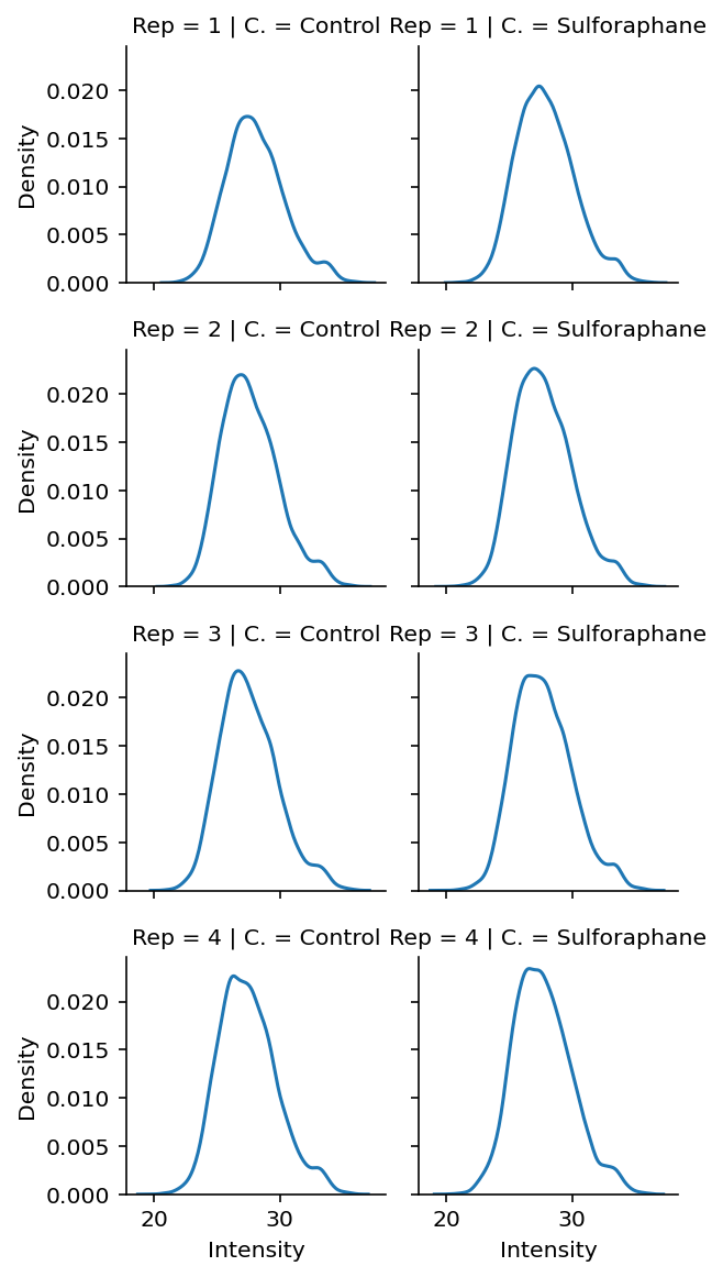
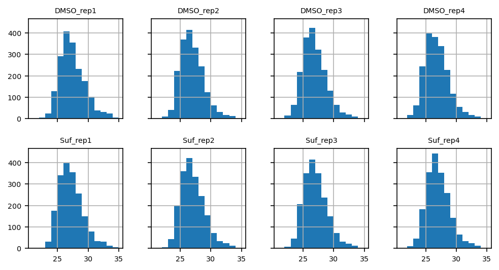
Exploratory and Data Quality Plots (peptide level)#
Shows the overal distribution of the log2-normal intensities per sample
df["BioReplicate"] = df["BioReplicate"].replace({5: 1, 6: 2, 7: 3, 8: 4})
fg = sns.displot(
data=df.rename(columns={"BioReplicate": "Rep", "Condition": "C."}),
x="Intensity",
col="C.",
row="Rep",
# hue="Reactor_ID",
kind="kde",
height=2,
aspect=1.1,
)
Aggregate the peptide intensities to protein intensities#
we use the median of the peptide intensities for each protein
There are more sophisticated ways to do this, e.g. using MaxLFQ, iBAQ, FlashLFQ, DirectLFQ, etc.
shorten sample name for readability
proteins = (
df.groupby(["ProteinName", "Reference"])["Intensity"].median().unstack(level=0)
)
proteins.index = proteins.index.str.split("_").str[4:6].str.join("_")
proteins
| ProteinName | CON_ENSEMBL:ENSBTAP00000024462;CON_ENSEMBL:ENSBTAP00000024466 | CON_O76013 | CON_P00761 | CON_P01966 | CON_P02070 | CON_P02533 | CON_P02538 | CON_P02662 | CON_P02663 | CON_P02666 | ... | sp|Q47319|TAPT_ECOLI | sp|Q47536|YAIP_ECOLI | sp|Q47622|SAPA_ECOLI | sp|Q47679|YAFV_ECOLI | sp|Q47710|YQJK_ECOLI | sp|Q57261|TRUD_ECOLI | sp|Q59385-2|COPA_ECOLI | sp|Q59385|COPA_ECOLI | sp|Q7DFV3|YMGG_ECOLI | sp|Q93K97|ADPP_ECOLI |
|---|---|---|---|---|---|---|---|---|---|---|---|---|---|---|---|---|---|---|---|---|---|
| Reference | |||||||||||||||||||||
| DMSO_rep1 | NaN | NaN | 31.055 | 24.202 | 26.890 | 28.336 | 25.828 | NaN | 26.762 | NaN | ... | NaN | NaN | 25.343 | NaN | 27.038 | 28.411 | 23.555 | 27.640 | 28.513 | 27.223 |
| DMSO_rep2 | NaN | 25.647 | 30.117 | 25.711 | NaN | 25.595 | 26.210 | NaN | 27.593 | NaN | ... | NaN | NaN | NaN | NaN | 26.841 | 27.941 | 25.240 | 27.244 | 27.621 | 25.291 |
| DMSO_rep3 | 25.529 | NaN | 33.767 | NaN | NaN | 26.992 | 25.441 | 28.129 | 28.895 | 29.559 | ... | NaN | NaN | 24.576 | NaN | 26.609 | 27.070 | NaN | 27.525 | 27.679 | 24.359 |
| DMSO_rep4 | NaN | NaN | 33.702 | NaN | NaN | 27.205 | 26.093 | NaN | 27.764 | NaN | ... | NaN | NaN | 25.945 | 23.902 | 27.164 | 26.680 | 22.524 | 27.404 | 27.256 | 25.767 |
| Suf_rep1 | NaN | NaN | 34.068 | NaN | NaN | NaN | 24.442 | NaN | 25.938 | NaN | ... | NaN | NaN | 25.836 | NaN | 26.819 | 27.995 | NaN | 27.499 | 28.090 | 25.956 |
| Suf_rep2 | NaN | NaN | 33.252 | NaN | 26.571 | 26.495 | 25.070 | NaN | NaN | NaN | ... | NaN | NaN | NaN | 24.162 | 27.268 | 27.055 | NaN | 27.667 | 27.526 | 25.231 |
| Suf_rep3 | NaN | NaN | 31.844 | 25.927 | NaN | 26.249 | 28.169 | 22.968 | 26.466 | NaN | ... | 25.463 | NaN | NaN | NaN | 24.741 | 27.313 | NaN | 27.708 | 27.814 | 26.103 |
| Suf_rep4 | NaN | NaN | 33.857 | NaN | NaN | 27.208 | 24.690 | NaN | NaN | NaN | ... | NaN | 24.468 | 24.757 | 24.040 | 27.071 | 26.643 | NaN | 27.848 | 27.605 | 26.178 |
8 rows × 2306 columns
Remove contaminant proteins#
Remove the contaminant proteins which were added to the fasta file used in the data processing. Contaminant proteins are e.g. creation which gets into the sample from the human skin or hair when the sample is prepared.
These are filtered out as they are most of the time not relevant, but a contamination.
decoy_proteins = proteins.filter(like="CON_", axis=1)
proteins = proteins.drop(decoy_proteins.columns, axis=1)
proteins
| ProteinName | sp|A5A613|YCIY_ECOLI | sp|P00350|6PGD_ECOLI | sp|P00363|FRDA_ECOLI | sp|P00370|DHE4_ECOLI | sp|P00393|NDH_ECOLI | sp|P00448|SODM_ECOLI | sp|P00452|RIR1_ECOLI | sp|P00490|PHSM_ECOLI | sp|P00509|AAT_ECOLI | sp|P00547|KHSE_ECOLI | ... | sp|Q47319|TAPT_ECOLI | sp|Q47536|YAIP_ECOLI | sp|Q47622|SAPA_ECOLI | sp|Q47679|YAFV_ECOLI | sp|Q47710|YQJK_ECOLI | sp|Q57261|TRUD_ECOLI | sp|Q59385-2|COPA_ECOLI | sp|Q59385|COPA_ECOLI | sp|Q7DFV3|YMGG_ECOLI | sp|Q93K97|ADPP_ECOLI |
|---|---|---|---|---|---|---|---|---|---|---|---|---|---|---|---|---|---|---|---|---|---|
| Reference | |||||||||||||||||||||
| DMSO_rep1 | 27.180 | 28.152 | 30.247 | 27.459 | 26.824 | 25.610 | NaN | 27.864 | 29.979 | 26.065 | ... | NaN | NaN | 25.343 | NaN | 27.038 | 28.411 | 23.555 | 27.640 | 28.513 | 27.223 |
| DMSO_rep2 | NaN | 27.926 | 30.262 | 26.873 | 26.757 | 24.901 | NaN | 26.439 | 29.048 | NaN | ... | NaN | NaN | NaN | NaN | 26.841 | 27.941 | 25.240 | 27.244 | 27.621 | 25.291 |
| DMSO_rep3 | NaN | 27.653 | 29.970 | 26.600 | 25.442 | 25.054 | 27.172 | 26.382 | 28.777 | NaN | ... | NaN | NaN | 24.576 | NaN | 26.609 | 27.070 | NaN | 27.525 | 27.679 | 24.359 |
| DMSO_rep4 | NaN | 27.152 | 29.471 | 26.439 | 25.799 | 24.790 | NaN | 26.820 | 29.485 | 25.524 | ... | NaN | NaN | 25.945 | 23.902 | 27.164 | 26.680 | 22.524 | 27.404 | 27.256 | 25.767 |
| Suf_rep1 | NaN | 27.442 | 30.005 | 27.400 | 26.671 | 25.564 | NaN | 27.685 | 29.295 | NaN | ... | NaN | NaN | 25.836 | NaN | 26.819 | 27.995 | NaN | 27.499 | 28.090 | 25.956 |
| Suf_rep2 | NaN | 27.032 | 30.086 | 27.189 | 26.886 | 25.378 | 27.364 | 27.531 | 29.284 | NaN | ... | NaN | NaN | NaN | 24.162 | 27.268 | 27.055 | NaN | 27.667 | 27.526 | 25.231 |
| Suf_rep3 | NaN | 27.815 | 29.904 | 27.139 | 26.711 | 25.318 | 26.062 | 27.545 | 29.357 | 26.265 | ... | 25.463 | NaN | NaN | NaN | 24.741 | 27.313 | NaN | 27.708 | 27.814 | 26.103 |
| Suf_rep4 | NaN | 27.587 | 29.575 | 27.224 | 26.321 | 25.360 | 25.101 | 27.705 | 29.584 | 26.427 | ... | NaN | 24.468 | 24.757 | 24.040 | 27.071 | 26.643 | NaN | 27.848 | 27.605 | 26.178 |
8 rows × 2269 columns
Factor variable#
Create a label for each sample based on the metadata.
we will use a string in the sample name, but you can see how the metadata is organized
This could be provided in a separate metadata file.
meta = df[["Condition", "BioReplicate", "Run", "Reference"]].drop_duplicates()
meta
| Condition | BioReplicate | Run | Reference | |
|---|---|---|---|---|
| 0 | Control | 1 | 1 | 20220830_JL-4884_Forster_Ecoli_DMSO_rep1_EG-1.... |
| 1 | Control | 2 | 2 | 20220830_JL-4884_Forster_Ecoli_DMSO_rep2_EG-2.... |
| 2 | Control | 3 | 3 | 20220830_JL-4884_Forster_Ecoli_DMSO_rep3_EG-3.... |
| 3 | Control | 4 | 4 | 20220830_JL-4884_Forster_Ecoli_DMSO_rep4_EG-4.... |
| 4 | Sulforaphane | 1 | 5 | 20220830_JL-4884_Forster_Ecoli_Suf_rep1_EG-5.mzML |
| 5 | Sulforaphane | 2 | 6 | 20220830_JL-4884_Forster_Ecoli_Suf_rep2_EG-6.mzML |
| 6 | Sulforaphane | 3 | 7 | 20220830_JL-4884_Forster_Ecoli_Suf_rep3_EG-7.mzML |
| 7 | Sulforaphane | 4 | 8 | 20220830_JL-4884_Forster_Ecoli_Suf_rep4_EG-8.mzML |
label_encoding = {0: "control", 1: "10 µm sulforaphane"}
label_suf = pd.Series(
proteins.index.str.contains("Suf_").astype(int),
index=proteins.index,
name="label_suf",
dtype=np.int8,
).map(label_encoding)
label_suf
Reference
DMSO_rep1 control
DMSO_rep2 control
DMSO_rep3 control
DMSO_rep4 control
Suf_rep1 10 µm sulforaphane
Suf_rep2 10 µm sulforaphane
Suf_rep3 10 µm sulforaphane
Suf_rep4 10 µm sulforaphane
Name: label_suf, dtype: object
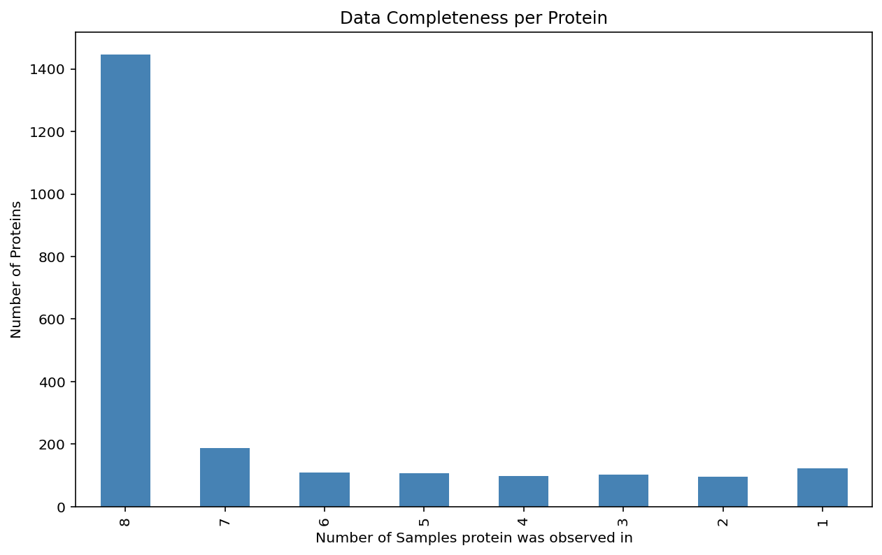
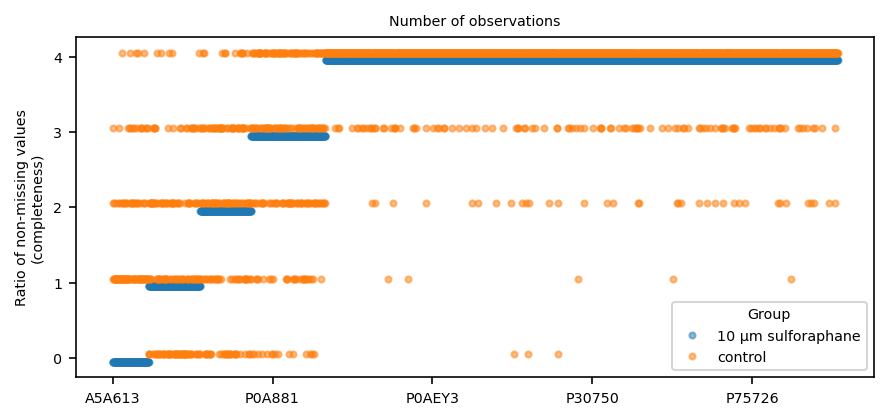
Plot the data completeness for each protein.#
see the how many proteins are observed across how many samples.
We create a subfolder in our results folder to keep it organized for the report generation later.
From the line plot (in staircase shape) you can see that over half of the proteins are observed in all 8 samples.
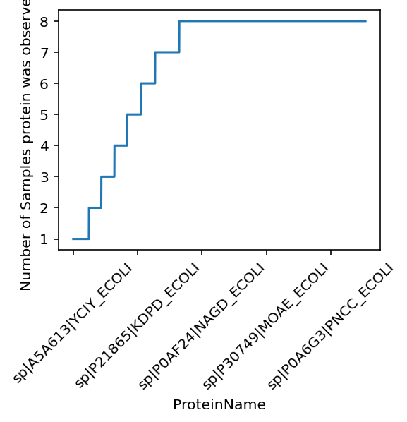
The bar plot shows the same information, but it is easier to see the exact number of proteins observed in how many samples.
Protein identifiers metadata#
Keep the protein identifiers metadata. Will be used to query UNIProt.
| Source | ProteinName | GeneName | |
|---|---|---|---|
| identifier | |||
| sp|A5A613|YCIY_ECOLI | sp | A5A613 | YCIY |
| sp|P00350|6PGD_ECOLI | sp | P00350 | 6PGD |
| sp|P00363|FRDA_ECOLI | sp | P00363 | FRDA |
| sp|P00370|DHE4_ECOLI | sp | P00370 | DHE4 |
| sp|P00393|NDH_ECOLI | sp | P00393 | NDH |
| ... | ... | ... | ... |
| sp|Q57261|TRUD_ECOLI | sp | Q57261 | TRUD |
| sp|Q59385-2|COPA_ECOLI | sp | Q59385-2 | COPA |
| sp|Q59385|COPA_ECOLI | sp | Q59385 | COPA |
| sp|Q7DFV3|YMGG_ECOLI | sp | Q7DFV3 | YMGG |
| sp|Q93K97|ADPP_ECOLI | sp | Q93K97 | ADPP |
2269 rows × 3 columns
For later in the enrichment analysis let’s replace the protein identifier from the Fasta file with the UNIPROT ID
proteins.columns = proteins_meta["ProteinName"].rename("UniprotID")
proteins
| UniprotID | A5A613 | P00350 | P00363 | P00370 | P00393 | P00448 | P00452 | P00490 | P00509 | P00547 | ... | Q47319 | Q47536 | Q47622 | Q47679 | Q47710 | Q57261 | Q59385-2 | Q59385 | Q7DFV3 | Q93K97 |
|---|---|---|---|---|---|---|---|---|---|---|---|---|---|---|---|---|---|---|---|---|---|
| Reference | |||||||||||||||||||||
| DMSO_rep1 | 27.180 | 28.152 | 30.247 | 27.459 | 26.824 | 25.610 | NaN | 27.864 | 29.979 | 26.065 | ... | NaN | NaN | 25.343 | NaN | 27.038 | 28.411 | 23.555 | 27.640 | 28.513 | 27.223 |
| DMSO_rep2 | NaN | 27.926 | 30.262 | 26.873 | 26.757 | 24.901 | NaN | 26.439 | 29.048 | NaN | ... | NaN | NaN | NaN | NaN | 26.841 | 27.941 | 25.240 | 27.244 | 27.621 | 25.291 |
| DMSO_rep3 | NaN | 27.653 | 29.970 | 26.600 | 25.442 | 25.054 | 27.172 | 26.382 | 28.777 | NaN | ... | NaN | NaN | 24.576 | NaN | 26.609 | 27.070 | NaN | 27.525 | 27.679 | 24.359 |
| DMSO_rep4 | NaN | 27.152 | 29.471 | 26.439 | 25.799 | 24.790 | NaN | 26.820 | 29.485 | 25.524 | ... | NaN | NaN | 25.945 | 23.902 | 27.164 | 26.680 | 22.524 | 27.404 | 27.256 | 25.767 |
| Suf_rep1 | NaN | 27.442 | 30.005 | 27.400 | 26.671 | 25.564 | NaN | 27.685 | 29.295 | NaN | ... | NaN | NaN | 25.836 | NaN | 26.819 | 27.995 | NaN | 27.499 | 28.090 | 25.956 |
| Suf_rep2 | NaN | 27.032 | 30.086 | 27.189 | 26.886 | 25.378 | 27.364 | 27.531 | 29.284 | NaN | ... | NaN | NaN | NaN | 24.162 | 27.268 | 27.055 | NaN | 27.667 | 27.526 | 25.231 |
| Suf_rep3 | NaN | 27.815 | 29.904 | 27.139 | 26.711 | 25.318 | 26.062 | 27.545 | 29.357 | 26.265 | ... | 25.463 | NaN | NaN | NaN | 24.741 | 27.313 | NaN | 27.708 | 27.814 | 26.103 |
| Suf_rep4 | NaN | 27.587 | 29.575 | 27.224 | 26.321 | 25.360 | 25.101 | 27.705 | 29.584 | 26.427 | ... | NaN | 24.468 | 24.757 | 24.040 | 27.071 | 26.643 | NaN | 27.848 | 27.605 | 26.178 |
8 rows × 2269 columns
And let’s save a table with the data for inspection
proteins_meta.to_csv(out_dir_subsection / "proteins_identifiers.csv")
proteins.to_csv(out_dir_subsection / "proteins.csv")
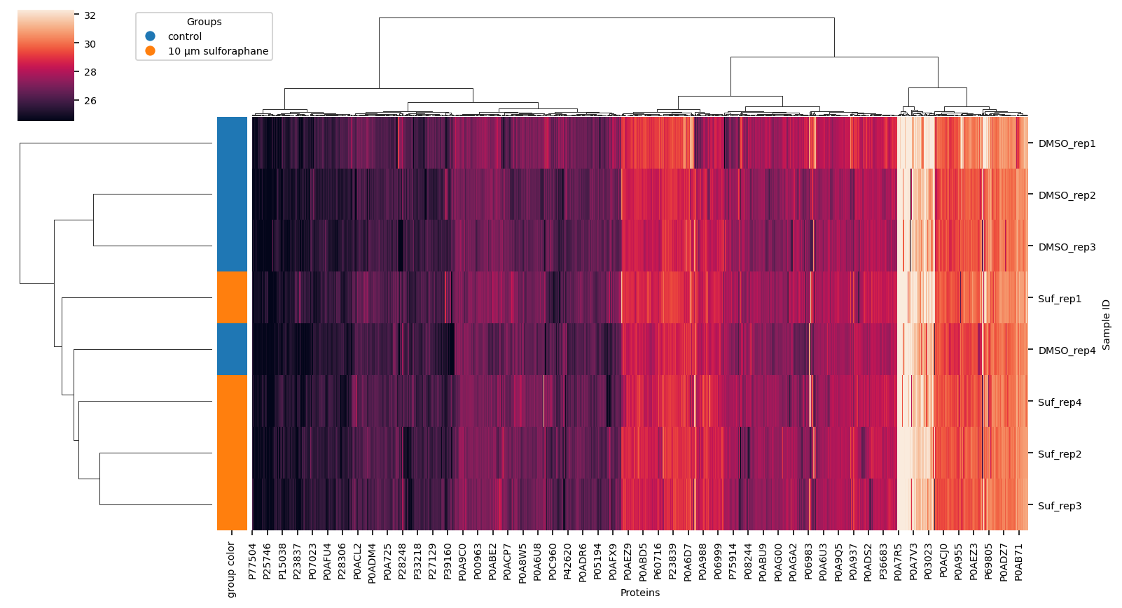
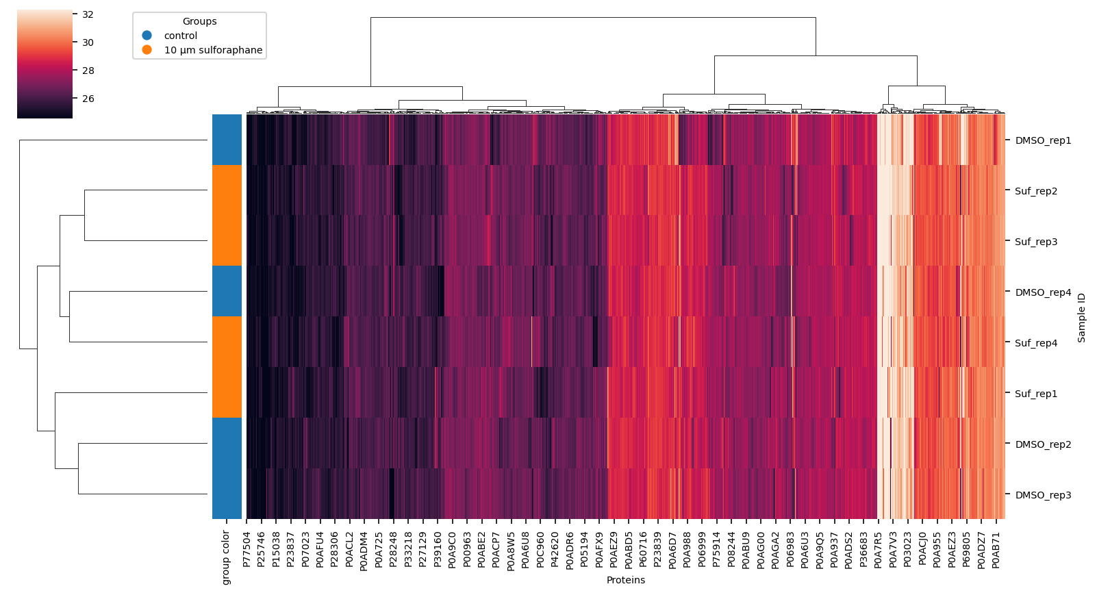
Hierarchical Clustering of data#
using completely observed data only find correlations in data
out_dir_subsection = out_dir / "1_data" / "clustermap"
out_dir_subsection.mkdir(parents=True, exist_ok=True)
_group_labels = label_encoding.values()
lut = dict(zip(_group_labels, [f"C{i}" for i in range(len(_group_labels))]))
row_colors = label_suf.map(lut).rename("group color")
row_colors
Reference
DMSO_rep1 C0
DMSO_rep2 C0
DMSO_rep3 C0
DMSO_rep4 C0
Suf_rep1 C1
Suf_rep2 C1
Suf_rep3 C1
Suf_rep4 C1
Name: group color, dtype: object
vuecore.set_font_sizes(7)
cg = sns.clustermap(
proteins.dropna(how="any", axis=1),
method="ward",
row_colors=row_colors,
figsize=(11, 6),
robust=True,
xticklabels=True,
yticklabels=True,
)
fig = cg.figure
cg.ax_heatmap.set_xlabel("Proteins")
cg.ax_heatmap.set_ylabel("Sample ID")
vuecore.select_xticks(cg.ax_heatmap)
handles = [
plt.Line2D([0], [0], marker="o", color="w", markerfacecolor=lut[name], markersize=8)
for name in lut
]
cg.ax_cbar.legend(
handles, _group_labels, title="Groups", loc="lower left", bbox_to_anchor=(2, 0.5)
)
fname = out_dir_subsection / "clustermap_ward.png"
# vuecore.savefig(fig, fname, pdf=True, dpi=600, tight_layout=False)
fig.savefig(
out_dir_subsection / "clustermap_ward.png",
bbox_inches="tight",
dpi=300,
)
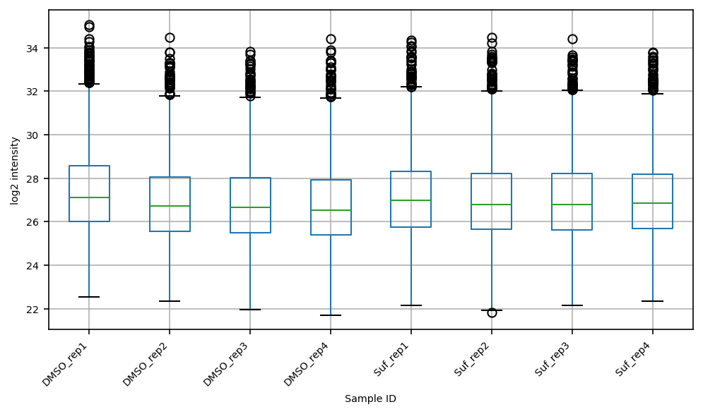
Quality Control Plots (protein level)#
data distribution (histogram and boxplot) to identify drift
coefficient of variation (CV)
number of identified proteins per sample
Data distribution (histogram)#
min_int, max_int = int(proteins.min().min()), int(proteins.max().max())
bins = range(min_int, max_int+1, 1)
ax = proteins.T.hist(layout=(2, 4), bins=bins, sharex=True, sharey=True, figsize=(8, 4))
Data distribution (boxplot)#
fig, ax = plt.subplots(figsize=(8, 4))
proteins.T.boxplot(ax=ax)
ax.set_xlabel("Sample ID")
ax.set_ylabel("log2 intensity")
ax.set_xticklabels(ax.get_xticklabels(), rotation=45, ha="right")
fname = out_dir_subsection / "boxplot_log2_unnormalized.png"
vuecore.savefig(fig, fname, pdf=True, dpi=600, tight_layout=False)
print(f"Saved boxplot to {fname}")
Saved boxplot to data/PXD040621/report/1_data/clustermap/boxplot_log2_unnormalized.png
Coefficient of Variation (CV)#
CV = standard deviation / mean $\( CV = \frac{\sigma}{\mu} \)$
per group
Use
scipy.stats.variation
to calculate the CV.
df_cvs = (
proteins.groupby(label_suf) # .join(metadata[grouping])
# .agg(scipy.stats.variation)
.agg([scipy.stats.variation, "mean"]) # .rename_axis(["feat", "stat"], axis=1)
)
df_cvs
| UniprotID | A5A613 | P00350 | P00363 | P00370 | P00393 | ... | Q57261 | Q59385-2 | Q59385 | Q7DFV3 | Q93K97 | ||||||||||
|---|---|---|---|---|---|---|---|---|---|---|---|---|---|---|---|---|---|---|---|---|---|
| variation | mean | variation | mean | variation | mean | variation | mean | variation | mean | ... | variation | mean | variation | mean | variation | mean | variation | mean | variation | mean | |
| label_suf | |||||||||||||||||||||
| 10 µm sulforaphane | NaN | NaN | 0.010 | 27.469 | 0.006 | 29.892 | 0.004 | 27.238 | 0.008 | 26.647 | ... | 0.018 | 27.252 | NaN | NaN | 0.004 | 27.680 | 0.008 | 27.759 | 0.015 | 25.867 |
| control | NaN | 27.180 | 0.013 | 27.721 | 0.011 | 29.987 | 0.014 | 26.843 | 0.023 | 26.205 | ... | 0.025 | 27.525 | NaN | 23.773 | 0.005 | 27.453 | 0.017 | 27.767 | 0.040 | 25.660 |
2 rows × 4538 columns
df_cvs = df_cvs.stack(0, future_stack=True).reset_index().dropna()
df_cvs
| label_suf | UniprotID | variation | mean | |
|---|---|---|---|---|
| 1 | 10 µm sulforaphane | P00350 | 0.010 | 27.469 |
| 2 | 10 µm sulforaphane | P00363 | 0.006 | 29.892 |
| 3 | 10 µm sulforaphane | P00370 | 0.004 | 27.238 |
| 4 | 10 µm sulforaphane | P00393 | 0.008 | 26.647 |
| 5 | 10 µm sulforaphane | P00448 | 0.004 | 25.405 |
| ... | ... | ... | ... | ... |
| 4,532 | control | Q47710 | 0.008 | 26.913 |
| 4,533 | control | Q57261 | 0.025 | 27.525 |
| 4,535 | control | Q59385 | 0.005 | 27.453 |
| 4,536 | control | Q7DFV3 | 0.017 | 27.767 |
| 4,537 | control | Q93K97 | 0.040 | 25.660 |
3144 rows × 4 columns
Visualize the relationship between the coefficient of variation (CV) and the mean intensity per group: x-axis: CV (‘variation’), y-axis: mean intensity.
Here no further filtering is needed, but many researchers filter for proteins with a mean intensity above a certain threshold (aroung 0.3). This is best done on quality control samples, e.g. a pooled sample, for large datasets.
Hierarchical Clustering of normalized data#
using completely observed data only Checkout the recipe on normalization methods.
Let’s see the effect of normalization on the clustering.
normalization_method = "median"
X = acore.normalization.normalize_data(
proteins.dropna(how="any", axis=1), normalization_method
)
# X = acore.normalization.normalize_data(
# X, "zscore"
# ) # to make it more comparable across proteins, but not necessary for the clustering
X
| UniprotID | P00350 | P00363 | P00370 | P00393 | P00448 | P00490 | P00509 | P00550 | P00561 | P00562 | ... | Q46868 | Q46893 | Q46920 | Q46948 | Q47147 | Q47710 | Q57261 | Q59385 | Q7DFV3 | Q93K97 |
|---|---|---|---|---|---|---|---|---|---|---|---|---|---|---|---|---|---|---|---|---|---|
| Reference | |||||||||||||||||||||
| DMSO_rep1 | 27.858 | 29.953 | 27.165 | 26.530 | 25.316 | 27.570 | 29.685 | 26.429 | 26.826 | 27.150 | ... | 29.139 | 27.865 | 27.059 | 26.919 | 26.365 | 26.744 | 28.117 | 27.346 | 28.219 | 26.929 |
| DMSO_rep2 | 28.064 | 30.399 | 27.011 | 26.894 | 25.039 | 26.576 | 29.185 | 25.603 | 26.598 | 26.720 | ... | 29.868 | 27.814 | 26.840 | 27.330 | 26.516 | 26.978 | 28.078 | 27.381 | 27.758 | 25.429 |
| DMSO_rep3 | 27.854 | 30.170 | 26.800 | 25.643 | 25.254 | 26.582 | 28.977 | 27.217 | 26.693 | 27.039 | ... | 29.720 | 28.852 | 27.007 | 27.230 | 26.680 | 26.809 | 27.271 | 27.725 | 27.879 | 24.559 |
| DMSO_rep4 | 27.319 | 29.638 | 26.606 | 25.966 | 24.957 | 26.987 | 29.652 | 26.835 | 26.685 | 26.529 | ... | 28.653 | 28.294 | 27.308 | 27.574 | 26.441 | 27.331 | 26.847 | 27.571 | 27.423 | 25.935 |
| Suf_rep1 | 27.261 | 29.824 | 27.219 | 26.490 | 25.383 | 27.504 | 29.114 | 26.637 | 26.764 | 27.028 | ... | 29.604 | 28.407 | 26.867 | 27.706 | 26.765 | 26.638 | 27.815 | 27.318 | 27.910 | 25.775 |
| Suf_rep2 | 27.029 | 30.084 | 27.187 | 26.884 | 25.375 | 27.529 | 29.281 | 27.030 | 27.099 | 26.015 | ... | 28.981 | 28.579 | 26.920 | 27.505 | 26.613 | 27.266 | 27.053 | 27.665 | 27.523 | 25.228 |
| Suf_rep3 | 27.817 | 29.907 | 27.141 | 26.714 | 25.321 | 27.548 | 29.359 | 27.011 | 26.773 | 26.364 | ... | 28.755 | 28.379 | 27.096 | 27.254 | 26.284 | 24.743 | 27.316 | 27.711 | 27.817 | 26.106 |
| Suf_rep4 | 27.533 | 29.521 | 27.169 | 26.266 | 25.306 | 27.650 | 29.529 | 26.921 | 26.931 | 26.808 | ... | 27.866 | 28.746 | 27.093 | 27.622 | 26.954 | 27.017 | 26.589 | 27.793 | 27.551 | 26.123 |
8 rows × 1446 columns
X.median(axis="columns")
Reference
DMSO_rep1 27.278
DMSO_rep2 27.278
DMSO_rep3 27.278
DMSO_rep4 27.278
Suf_rep1 27.278
Suf_rep2 27.278
Suf_rep3 27.278
Suf_rep4 27.278
dtype: float64
Exercise:
Try out different normalization methods and see how the clustering changes.
Maybe you want to combine a sample based with a protein based normalization method.
Differential Regulation#
out_dir_subsection = out_dir / "2_differential_regulation"
out_dir_subsection.mkdir(parents=True, exist_ok=True)
Retain all proteins with at least 3 observations in each group
this is a requirement for a standard t-test
you could look into imputation methods to fill in missing values)
protein in at least two samples per group?
missing all in one condition?
Let’s not impute, but filter for proteins with at least 3 observations in each group
group_counts = proteins.groupby(label_suf).count()
group_counts
| UniprotID | A5A613 | P00350 | P00363 | P00370 | P00393 | P00448 | P00452 | P00490 | P00509 | P00547 | ... | Q47319 | Q47536 | Q47622 | Q47679 | Q47710 | Q57261 | Q59385-2 | Q59385 | Q7DFV3 | Q93K97 |
|---|---|---|---|---|---|---|---|---|---|---|---|---|---|---|---|---|---|---|---|---|---|
| label_suf | |||||||||||||||||||||
| 10 µm sulforaphane | 0 | 4 | 4 | 4 | 4 | 4 | 3 | 4 | 4 | 2 | ... | 1 | 1 | 2 | 2 | 4 | 4 | 0 | 4 | 4 | 4 |
| control | 1 | 4 | 4 | 4 | 4 | 4 | 1 | 4 | 4 | 2 | ... | 0 | 0 | 3 | 1 | 4 | 4 | 3 | 4 | 4 | 4 |
2 rows × 2269 columns
Let’s see how many observations are present by condition (group)
The order is dermined by the treatment group here
Some proteins are absent in the control group that are observed in the treatment group, which is interesting for a separate analysis (not shown).
Text(0.5, 1.0, 'Number of observations')
For now, we filter the proteins to only those with at least 3 observations in each group.
mask = group_counts.groupby("label_suf").transform(
lambda x: x >= min_obs_per_group
).all(axis=0)
mask
UniprotID
A5A613 False
P00350 True
P00363 True
P00370 True
P00393 True
...
Q57261 True
Q59385-2 False
Q59385 True
Q7DFV3 True
Q93K97 True
Length: 2269, dtype: bool
We use a simple t-test for the differential regulation analysis.
Experiment with the normalization method and it’s effect on the results.
view = X.loc[:, mask].join(label_suf)
group = label_suf.name
diff_reg = acore.differential_regulation.run_anova(
view,
alpha=0.15,
drop_cols=[],
subject=None,
group=group,
).sort_values("pvalue", ascending=True)
diff_reg["rejected"] = diff_reg["rejected"].astype(bool)
diff_reg.sort_values("pvalue")
| identifier | T-Statistics | pvalue | mean(group1) | mean(group2) | std(group1) | std(group2) | log2FC | test | correction | padj | rejected | group1 | group2 | FC | -log10 pvalue | Method | |
|---|---|---|---|---|---|---|---|---|---|---|---|---|---|---|---|---|---|
| 1,321 | P75726 | 13.440 | 0.000 | 28.135 | 26.793 | 0.131 | 0.113 | 1.341 | t-Test | FDR correction BH | 0.015 | True | control | 10 µm sulforaphane | 2.534 | 4.978 | Unpaired t-test |
| 1,375 | P76440 | 10.610 | 0.000 | 27.235 | 26.580 | 0.082 | 0.068 | 0.655 | t-Test | FDR correction BH | 0.030 | True | control | 10 µm sulforaphane | 1.575 | 4.384 | Unpaired t-test |
| 827 | P0CK95 | -9.341 | 0.000 | 26.461 | 27.223 | 0.126 | 0.063 | -0.762 | t-Test | FDR correction BH | 0.032 | True | control | 10 µm sulforaphane | 0.590 | 4.069 | Unpaired t-test |
| 513 | P0ABK5 | -8.911 | 0.000 | 29.683 | 30.465 | 0.064 | 0.138 | -0.783 | t-Test | FDR correction BH | 0.032 | True | control | 10 µm sulforaphane | 0.581 | 3.953 | Unpaired t-test |
| 35 | P02943 | -8.791 | 0.000 | 26.170 | 27.861 | 0.282 | 0.178 | -1.691 | t-Test | FDR correction BH | 0.032 | True | control | 10 µm sulforaphane | 0.310 | 3.920 | Unpaired t-test |
| ... | ... | ... | ... | ... | ... | ... | ... | ... | ... | ... | ... | ... | ... | ... | ... | ... | ... |
| 101 | P07650 | -0.003 | 0.998 | 27.861 | 27.861 | 0.191 | 0.123 | -0.000 | t-Test | FDR correction BH | 0.999 | False | control | 10 µm sulforaphane | 1.000 | 0.001 | Unpaired t-test |
| 47 | P04846 | 0.002 | 0.998 | 25.750 | 25.749 | 0.086 | 0.285 | 0.000 | t-Test | FDR correction BH | 0.999 | False | control | 10 µm sulforaphane | 1.000 | 0.001 | Unpaired t-test |
| 1,038 | P31120 | -0.001 | 0.999 | 28.647 | 28.647 | 0.106 | 0.087 | -0.000 | t-Test | FDR correction BH | 0.999 | False | control | 10 µm sulforaphane | 1.000 | 0.000 | Unpaired t-test |
| 1,291 | P67660 | 0.001 | 0.999 | 26.369 | 26.368 | 0.210 | 0.269 | 0.000 | t-Test | FDR correction BH | 0.999 | False | control | 10 µm sulforaphane | 1.000 | 0.000 | Unpaired t-test |
| 774 | P0AG24 | 0.001 | 0.999 | 25.513 | 25.513 | 0.858 | 0.175 | 0.001 | t-Test | FDR correction BH | 0.999 | False | control | 10 µm sulforaphane | 1.000 | 0.000 | Unpaired t-test |
1446 rows × 17 columns
diff_reg.sort_values("pvalue").head(20)
| identifier | T-Statistics | pvalue | mean(group1) | mean(group2) | std(group1) | std(group2) | log2FC | test | correction | padj | rejected | group1 | group2 | FC | -log10 pvalue | Method | |
|---|---|---|---|---|---|---|---|---|---|---|---|---|---|---|---|---|---|
| 1,321 | P75726 | 13.440 | 0.000 | 28.135 | 26.793 | 0.131 | 0.113 | 1.341 | t-Test | FDR correction BH | 0.015 | True | control | 10 µm sulforaphane | 2.534 | 4.978 | Unpaired t-test |
| 1,375 | P76440 | 10.610 | 0.000 | 27.235 | 26.580 | 0.082 | 0.068 | 0.655 | t-Test | FDR correction BH | 0.030 | True | control | 10 µm sulforaphane | 1.575 | 4.384 | Unpaired t-test |
| 827 | P0CK95 | -9.341 | 0.000 | 26.461 | 27.223 | 0.126 | 0.063 | -0.762 | t-Test | FDR correction BH | 0.032 | True | control | 10 µm sulforaphane | 0.590 | 4.069 | Unpaired t-test |
| 513 | P0ABK5 | -8.911 | 0.000 | 29.683 | 30.465 | 0.064 | 0.138 | -0.783 | t-Test | FDR correction BH | 0.032 | True | control | 10 µm sulforaphane | 0.581 | 3.953 | Unpaired t-test |
| 35 | P02943 | -8.791 | 0.000 | 26.170 | 27.861 | 0.282 | 0.178 | -1.691 | t-Test | FDR correction BH | 0.032 | True | control | 10 µm sulforaphane | 0.310 | 3.920 | Unpaired t-test |
| 1,431 | Q46835 | -8.614 | 0.000 | 26.776 | 27.618 | 0.124 | 0.115 | -0.842 | t-Test | FDR correction BH | 0.032 | True | control | 10 µm sulforaphane | 0.558 | 3.871 | Unpaired t-test |
| 832 | P10384 | -6.345 | 0.001 | 26.482 | 27.416 | 0.213 | 0.140 | -0.934 | t-Test | FDR correction BH | 0.147 | True | control | 10 µm sulforaphane | 0.524 | 3.144 | Unpaired t-test |
| 129 | P09152 | 6.197 | 0.001 | 26.875 | 26.191 | 0.074 | 0.176 | 0.684 | t-Test | FDR correction BH | 0.147 | True | control | 10 µm sulforaphane | 1.607 | 3.090 | Unpaired t-test |
| 1,237 | P60785 | -5.771 | 0.001 | 28.240 | 28.460 | 0.056 | 0.035 | -0.220 | t-Test | FDR correction BH | 0.164 | False | control | 10 µm sulforaphane | 0.859 | 2.928 | Unpaired t-test |
| 1,113 | P37349 | 5.711 | 0.001 | 25.988 | 25.193 | 0.235 | 0.053 | 0.795 | t-Test | FDR correction BH | 0.164 | False | control | 10 µm sulforaphane | 1.735 | 2.904 | Unpaired t-test |
| 991 | P27249 | -5.709 | 0.001 | 24.921 | 25.351 | 0.067 | 0.112 | -0.430 | t-Test | FDR correction BH | 0.164 | False | control | 10 µm sulforaphane | 0.742 | 2.903 | Unpaired t-test |
| 487 | P0AB67 | -5.519 | 0.001 | 27.878 | 28.381 | 0.089 | 0.131 | -0.503 | t-Test | FDR correction BH | 0.179 | False | control | 10 µm sulforaphane | 0.705 | 2.827 | Unpaired t-test |
| 514 | P0ABK9 | 5.370 | 0.002 | 26.416 | 25.578 | 0.147 | 0.226 | 0.838 | t-Test | FDR correction BH | 0.190 | False | control | 10 µm sulforaphane | 1.787 | 2.767 | Unpaired t-test |
| 1,329 | P75825 | 4.990 | 0.002 | 26.956 | 25.320 | 0.220 | 0.524 | 1.636 | t-Test | FDR correction BH | 0.236 | False | control | 10 µm sulforaphane | 3.109 | 2.606 | Unpaired t-test |
| 959 | P25437 | -4.910 | 0.003 | 29.141 | 29.686 | 0.181 | 0.064 | -0.545 | t-Test | FDR correction BH | 0.236 | False | control | 10 µm sulforaphane | 0.685 | 2.571 | Unpaired t-test |
| 1,394 | P77252 | 4.851 | 0.003 | 26.593 | 25.953 | 0.119 | 0.195 | 0.639 | t-Test | FDR correction BH | 0.236 | False | control | 10 µm sulforaphane | 1.558 | 2.545 | Unpaired t-test |
| 27 | P00968 | -4.802 | 0.003 | 26.452 | 26.880 | 0.083 | 0.130 | -0.429 | t-Test | FDR correction BH | 0.236 | False | control | 10 µm sulforaphane | 0.743 | 2.524 | Unpaired t-test |
| 110 | P08200 | -4.789 | 0.003 | 28.812 | 29.396 | 0.182 | 0.107 | -0.584 | t-Test | FDR correction BH | 0.236 | False | control | 10 µm sulforaphane | 0.667 | 2.518 | Unpaired t-test |
| 562 | P0ACD8 | 4.767 | 0.003 | 30.243 | 29.895 | 0.090 | 0.089 | 0.348 | t-Test | FDR correction BH | 0.236 | False | control | 10 µm sulforaphane | 1.273 | 2.508 | Unpaired t-test |
| 399 | P0A9I1 | 4.499 | 0.004 | 28.152 | 26.938 | 0.357 | 0.301 | 1.214 | t-Test | FDR correction BH | 0.280 | False | control | 10 µm sulforaphane | 2.320 | 2.387 | Unpaired t-test |
Interactive Volcano Plot#
y-axis: -log10(p-value)
x-axis: log2(fold-change)
color: rejected (significant or not after multiple testing correction)
Hover over the points to see additional information
Save result to subsection folder
fig.write_json(
out_dir_subsection / "0_volcano_plot.json",
pretty=False,
)
diff_reg.to_csv(out_dir_subsection / "1_differential_regulation.csv")
Enrichment Analysis#
You can reload the annotations, but for latency, I added a cached version to the repository
out_dir_subsection = out_dir / "uniprot_annotations"
out_dir_subsection.mkdir(parents=True, exist_ok=True)
Fetch the annotations from UniProt API.#
fname_annotations = out_dir_subsection / "annotations.csv"
try:
annotations = pd.read_csv(fname_annotations, index_col=0)
print(f"Loaded annotations from {fname_annotations}")
except FileNotFoundError:
print(f"Fetching annotations for {proteins.columns.size} UniProt IDs.")
FIELDS = "go_p,go_c,go_f"
annotations = fetch_annotations(proteins.columns, fields=FIELDS)
annotations = process_annotations(annotations, fields=FIELDS)
# cache the annotations
fname_annotations.parent.mkdir(exist_ok=True, parents=True)
annotations.to_csv(fname_annotations, index=True)
annotations
Loaded annotations from data/PXD040621/report/uniprot_annotations/annotations.csv
| identifier | source | annotation | |
|---|---|---|---|
| 6 | P00350 | Gene Ontology (biological process) | D-gluconate catabolic process [GO:0046177] |
| 7 | P00350 | Gene Ontology (cellular component) | cytosol [GO:0005829] |
| 8 | P00350 | Gene Ontology (molecular function) | guanosine tetraphosphate binding [GO:0097216] |
| 9 | P00350 | Gene Ontology (molecular function) | identical protein binding [GO:0042802] |
| 10 | P00350 | Gene Ontology (molecular function) | NADP binding [GO:0050661] |
| ... | ... | ... | ... |
| 32,263 | ADPP_ECOLI | Gene Ontology (molecular function) | magnesium ion binding [GO:0000287] |
| 32,264 | ADPP_ECOLI | Gene Ontology (molecular function) | protein homodimerization activity [GO:0042803] |
| 32,265 | ADPP_ECOLI | Gene Ontology (molecular function) | pyrophosphatase activity [GO:0016462] |
| 32,266 | ADPP_ECOLI | Gene Ontology (biological process) | response to heat [GO:0009408] |
| 32,267 | ADPP_ECOLI | Gene Ontology (biological process) | ribose phosphate metabolic process [GO:0019693] |
30283 rows × 3 columns
Run the enrichment analysis#
background is the set of identified proteins in the experiment (not the whole proteome of the organisim, here E. coli)
The enrichment is performed separately for the up- and down-regulated proteins (‘rejected’), which are few in our example where we had to set the adjusted p-value to 0.15.
In the enrichment we set the cutoff for the adjusted p-value to 0.2, which is a bit arbitrary to see some results.
enriched = acore.enrichment_analysis.run_up_down_regulation_enrichment(
regulation_data=diff_reg,
annotation=annotations,
min_detected_in_set=1,
lfc_cutoff=1,
pval_col="padj", # toggle if it does not work
correction_alpha=0.2, # adjust the p-value to see more or less results
)
enriched.set_index('identifiers')
| terms | foreground | background | foreground_pop | background_pop | pvalue | padj | rejected | direction | comparison | |
|---|---|---|---|---|---|---|---|---|---|---|
| identifiers | ||||||||||
| P75726 | citrate CoA-transferase activity [GO:0008814] | 1 | 0 | 1 | 1446 | 0.001 | 0.002 | True | upregulated | control~10 µm sulforaphane |
| P75726 | citrate metabolic process [GO:0006101] | 1 | 1 | 1 | 1446 | 0.001 | 0.002 | True | upregulated | control~10 µm sulforaphane |
| P75726 | ATP-independent citrate lyase complex [GO:0009... | 1 | 1 | 1 | 1446 | 0.001 | 0.002 | True | upregulated | control~10 µm sulforaphane |
| P75726 | acetyl-CoA metabolic process [GO:0006084] | 1 | 1 | 1 | 1446 | 0.001 | 0.002 | True | upregulated | control~10 µm sulforaphane |
| P75726 | citrate (pro-3S)-lyase activity [GO:0008815] | 1 | 1 | 1 | 1446 | 0.001 | 0.002 | True | upregulated | control~10 µm sulforaphane |
| P75726 | cytoplasm [GO:0005737] | 1 | 28 | 1 | 1446 | 0.020 | 0.020 | True | upregulated | control~10 µm sulforaphane |
| P02943 | maltodextrin transmembrane transporter activi... | 1 | 0 | 1 | 1446 | 0.001 | 0.002 | True | downregulated | control~10 µm sulforaphane |
| P02943 | maltose transmembrane transport [GO:1904981] | 1 | 0 | 1 | 1446 | 0.001 | 0.002 | True | downregulated | control~10 µm sulforaphane |
| P02943 | maltose transmembrane transporter activity [G... | 1 | 0 | 1 | 1446 | 0.001 | 0.002 | True | downregulated | control~10 µm sulforaphane |
| P02943 | maltose transporting porin activity [GO:0015481] | 1 | 0 | 1 | 1446 | 0.001 | 0.002 | True | downregulated | control~10 µm sulforaphane |
| P02943 | polysaccharide transport [GO:0015774] | 1 | 0 | 1 | 1446 | 0.001 | 0.002 | True | downregulated | control~10 µm sulforaphane |
| P02943 | maltodextrin transmembrane transport [GO:0042... | 1 | 1 | 1 | 1446 | 0.001 | 0.002 | True | downregulated | control~10 µm sulforaphane |
| P02943 | carbohydrate transmembrane transporter activit... | 1 | 1 | 1 | 1446 | 0.001 | 0.002 | True | downregulated | control~10 µm sulforaphane |
| P02943 | virus receptor activity [GO:0001618] | 1 | 1 | 1 | 1446 | 0.001 | 0.002 | True | downregulated | control~10 µm sulforaphane |
| P02943 | outer membrane protein complex [GO:0106234] | 1 | 2 | 1 | 1446 | 0.002 | 0.003 | True | downregulated | control~10 µm sulforaphane |
| P02943 | monoatomic ion transport [GO:0006811] | 1 | 2 | 1 | 1446 | 0.002 | 0.003 | True | downregulated | control~10 µm sulforaphane |
| P02943 | porin activity [GO:0015288] | 1 | 5 | 1 | 1446 | 0.004 | 0.005 | True | downregulated | control~10 µm sulforaphane |
| P02943 | pore complex [GO:0046930] | 1 | 5 | 1 | 1446 | 0.004 | 0.005 | True | downregulated | control~10 µm sulforaphane |
| P02943 | cell outer membrane [GO:0009279] | 1 | 37 | 1 | 1446 | 0.026 | 0.028 | True | downregulated | control~10 µm sulforaphane |
| P02943 | DNA damage response [GO:0006974] | 1 | 42 | 1 | 1446 | 0.030 | 0.030 | True | downregulated | control~10 µm sulforaphane |
Plot the enrichment scores for the up- and down-regulated proteins separately.
y-axis: GO term
x-axis: enrichment score (e.g. -log10(p-pvalue adjusted))
Check for Maltose Uptake#
out_dir_subsection = out_dir / "3_maltose_uptake"
out_dir_subsection.mkdir(parents=True, exist_ok=True)
Apply filtering of ‘differentially abundant proteins’ as described in the paper
“Differentially abundant proteins were determined as those with log2 fold-change \(log2FC > 1\) and \(log2FC < -1\), and \(p < 0.05\)”
This means no multiple testing correction was applied.
view = diff_reg.query("pvalue < 0.05 and FC > 1") # .shape[0]
view.to_csv(
out_dir_subsection / "1_differently_regulated_as_in_paper.csv",
index=False,
)
view.set_index("identifier")[['pvalue', 'log2FC', 'padj', 'rejected', 'mean(group1)', 'mean(group2)',
'std(group1)', 'std(group2)', 'test', 'correction',
'group1', 'group2', 'FC', '-log10 pvalue', 'Method']]
| pvalue | log2FC | padj | rejected | mean(group1) | mean(group2) | std(group1) | std(group2) | test | correction | group1 | group2 | FC | -log10 pvalue | Method | |
|---|---|---|---|---|---|---|---|---|---|---|---|---|---|---|---|
| identifier | |||||||||||||||
| P75726 | 0.000 | 1.341 | 0.015 | True | 28.135 | 26.793 | 0.131 | 0.113 | t-Test | FDR correction BH | control | 10 µm sulforaphane | 2.534 | 4.978 | Unpaired t-test |
| P76440 | 0.000 | 0.655 | 0.030 | True | 27.235 | 26.580 | 0.082 | 0.068 | t-Test | FDR correction BH | control | 10 µm sulforaphane | 1.575 | 4.384 | Unpaired t-test |
| P09152 | 0.001 | 0.684 | 0.147 | True | 26.875 | 26.191 | 0.074 | 0.176 | t-Test | FDR correction BH | control | 10 µm sulforaphane | 1.607 | 3.090 | Unpaired t-test |
| P37349 | 0.001 | 0.795 | 0.164 | False | 25.988 | 25.193 | 0.235 | 0.053 | t-Test | FDR correction BH | control | 10 µm sulforaphane | 1.735 | 2.904 | Unpaired t-test |
| P0ABK9 | 0.002 | 0.838 | 0.190 | False | 26.416 | 25.578 | 0.147 | 0.226 | t-Test | FDR correction BH | control | 10 µm sulforaphane | 1.787 | 2.767 | Unpaired t-test |
| P75825 | 0.002 | 1.636 | 0.236 | False | 26.956 | 25.320 | 0.220 | 0.524 | t-Test | FDR correction BH | control | 10 µm sulforaphane | 3.109 | 2.606 | Unpaired t-test |
| P77252 | 0.003 | 0.639 | 0.236 | False | 26.593 | 25.953 | 0.119 | 0.195 | t-Test | FDR correction BH | control | 10 µm sulforaphane | 1.558 | 2.545 | Unpaired t-test |
| P0ACD8 | 0.003 | 0.348 | 0.236 | False | 30.243 | 29.895 | 0.090 | 0.089 | t-Test | FDR correction BH | control | 10 µm sulforaphane | 1.273 | 2.508 | Unpaired t-test |
| P0A9I1 | 0.004 | 1.214 | 0.280 | False | 28.152 | 26.938 | 0.357 | 0.301 | t-Test | FDR correction BH | control | 10 µm sulforaphane | 2.320 | 2.387 | Unpaired t-test |
| P0A7E3 | 0.005 | 0.816 | 0.288 | False | 27.388 | 26.572 | 0.072 | 0.317 | t-Test | FDR correction BH | control | 10 µm sulforaphane | 1.760 | 2.317 | Unpaired t-test |
| P19931 | 0.006 | 0.605 | 0.345 | False | 27.319 | 26.714 | 0.109 | 0.232 | t-Test | FDR correction BH | control | 10 µm sulforaphane | 1.521 | 2.189 | Unpaired t-test |
| P05637 | 0.009 | 0.699 | 0.369 | False | 26.674 | 25.975 | 0.131 | 0.288 | t-Test | FDR correction BH | control | 10 µm sulforaphane | 1.623 | 2.062 | Unpaired t-test |
| P25397 | 0.009 | 0.741 | 0.385 | False | 27.685 | 26.944 | 0.205 | 0.271 | t-Test | FDR correction BH | control | 10 µm sulforaphane | 1.671 | 2.031 | Unpaired t-test |
| P37637 | 0.013 | 0.326 | 0.468 | False | 28.952 | 28.626 | 0.130 | 0.096 | t-Test | FDR correction BH | control | 10 µm sulforaphane | 1.254 | 1.888 | Unpaired t-test |
| P24232 | 0.014 | 0.923 | 0.470 | False | 27.189 | 26.266 | 0.418 | 0.203 | t-Test | FDR correction BH | control | 10 µm sulforaphane | 1.896 | 1.860 | Unpaired t-test |
| P37765 | 0.015 | 0.359 | 0.495 | False | 27.570 | 27.211 | 0.032 | 0.182 | t-Test | FDR correction BH | control | 10 µm sulforaphane | 1.283 | 1.822 | Unpaired t-test |
| P68767 | 0.016 | 0.589 | 0.510 | False | 28.552 | 27.963 | 0.128 | 0.279 | t-Test | FDR correction BH | control | 10 µm sulforaphane | 1.504 | 1.799 | Unpaired t-test |
| P0AGL2 | 0.019 | 0.420 | 0.586 | False | 30.640 | 30.221 | 0.105 | 0.203 | t-Test | FDR correction BH | control | 10 µm sulforaphane | 1.338 | 1.721 | Unpaired t-test |
| P31142 | 0.022 | 1.073 | 0.624 | False | 28.163 | 27.090 | 0.122 | 0.590 | t-Test | FDR correction BH | control | 10 µm sulforaphane | 2.103 | 1.667 | Unpaired t-test |
| P69811 | 0.022 | 0.636 | 0.624 | False | 29.010 | 28.374 | 0.094 | 0.347 | t-Test | FDR correction BH | control | 10 µm sulforaphane | 1.554 | 1.657 | Unpaired t-test |
| P24228 | 0.025 | 0.794 | 0.674 | False | 25.663 | 24.869 | 0.304 | 0.348 | t-Test | FDR correction BH | control | 10 µm sulforaphane | 1.734 | 1.605 | Unpaired t-test |
| P11349 | 0.025 | 0.632 | 0.674 | False | 27.512 | 26.880 | 0.367 | 0.032 | t-Test | FDR correction BH | control | 10 µm sulforaphane | 1.550 | 1.603 | Unpaired t-test |
| P37127 | 0.025 | 0.673 | 0.674 | False | 25.256 | 24.583 | 0.085 | 0.384 | t-Test | FDR correction BH | control | 10 µm sulforaphane | 1.595 | 1.599 | Unpaired t-test |
| P0A6W9 | 0.028 | 0.834 | 0.677 | False | 27.536 | 26.702 | 0.302 | 0.401 | t-Test | FDR correction BH | control | 10 µm sulforaphane | 1.783 | 1.553 | Unpaired t-test |
| P69829 | 0.030 | 0.733 | 0.677 | False | 26.959 | 26.226 | 0.216 | 0.395 | t-Test | FDR correction BH | control | 10 µm sulforaphane | 1.662 | 1.518 | Unpaired t-test |
| P0AB52 | 0.035 | 2.149 | 0.733 | False | 28.457 | 26.308 | 1.055 | 0.877 | t-Test | FDR correction BH | control | 10 µm sulforaphane | 4.435 | 1.457 | Unpaired t-test |
| P63235 | 0.038 | 0.878 | 0.733 | False | 30.551 | 29.673 | 0.290 | 0.497 | t-Test | FDR correction BH | control | 10 µm sulforaphane | 1.837 | 1.415 | Unpaired t-test |
| P16659 | 0.039 | 0.422 | 0.733 | False | 29.434 | 29.012 | 0.263 | 0.089 | t-Test | FDR correction BH | control | 10 µm sulforaphane | 1.339 | 1.407 | Unpaired t-test |
| P18390 | 0.041 | 0.856 | 0.733 | False | 26.130 | 25.274 | 0.401 | 0.406 | t-Test | FDR correction BH | control | 10 µm sulforaphane | 1.809 | 1.390 | Unpaired t-test |
| P0AE74 | 0.041 | 0.984 | 0.733 | False | 26.505 | 25.521 | 0.643 | 0.138 | t-Test | FDR correction BH | control | 10 µm sulforaphane | 1.978 | 1.385 | Unpaired t-test |
| P37773 | 0.043 | 0.718 | 0.735 | False | 27.938 | 27.221 | 0.149 | 0.463 | t-Test | FDR correction BH | control | 10 µm sulforaphane | 1.644 | 1.365 | Unpaired t-test |
| P0AE45 | 0.046 | 1.216 | 0.768 | False | 26.325 | 25.110 | 0.516 | 0.660 | t-Test | FDR correction BH | control | 10 µm sulforaphane | 2.323 | 1.340 | Unpaired t-test |
| P0AGI8 | 0.047 | 0.640 | 0.773 | False | 26.223 | 25.583 | 0.422 | 0.142 | t-Test | FDR correction BH | control | 10 µm sulforaphane | 1.558 | 1.325 | Unpaired t-test |
| P0AET5 | 0.048 | 0.393 | 0.773 | False | 30.623 | 30.230 | 0.267 | 0.063 | t-Test | FDR correction BH | control | 10 µm sulforaphane | 1.313 | 1.322 | Unpaired t-test |
| P30850 | 0.048 | 0.526 | 0.773 | False | 28.148 | 27.623 | 0.142 | 0.338 | t-Test | FDR correction BH | control | 10 µm sulforaphane | 1.440 | 1.322 | Unpaired t-test |
| P06961 | 0.049 | 0.303 | 0.773 | False | 25.429 | 25.126 | 0.135 | 0.166 | t-Test | FDR correction BH | control | 10 µm sulforaphane | 1.234 | 1.306 | Unpaired t-test |
Let’s find the proteins highlighted in the volcano plot in Figure 3 in the
paper:

| Source | ProteinName | GeneName | |
|---|---|---|---|
| identifier | |||
| sp|P00363|FRDA_ECOLI | sp | P00363 | FRDA |
| sp|P02943|LAMB_ECOLI | sp | P02943 | LAMB |
| sp|P0A8Q0|FRDC_ECOLI | sp | P0A8Q0 | FRDC |
| sp|P0A8Q3|FRDD_ECOLI | sp | P0A8Q3 | FRDD |
| sp|P0A9I1|CITE_ECOLI | sp | P0A9I1 | CITE |
| sp|P0AC47|FRDB_ECOLI | sp | P0AC47 | FRDB |
| sp|P0AE74|CITT_ECOLI | sp | P0AE74 | CITT |
| sp|P0AEX9|MALE_ECOLI | sp | P0AEX9 | MALE |
| sp|P68187|MALK_ECOLI | sp | P68187 | MALK |
| GeneName | log2FC | pvalue | padj | rejected | group1 | group2 | Method | |
|---|---|---|---|---|---|---|---|---|
| identifier | ||||||||
| P0A9I1 | CITE | 1.214 | 0.004 | 0.280 | False | control | 10 µm sulforaphane | Unpaired t-test |
| P0AE74 | CITT | 0.984 | 0.041 | 0.733 | False | control | 10 µm sulforaphane | Unpaired t-test |
| P0A8Q0 | FRDC | 0.927 | 0.114 | 0.833 | False | control | 10 µm sulforaphane | Unpaired t-test |
| P00363 | FRDA | 0.206 | 0.342 | 0.855 | False | control | 10 µm sulforaphane | Unpaired t-test |
| P0AC47 | FRDB | 0.174 | 0.383 | 0.866 | False | control | 10 µm sulforaphane | Unpaired t-test |
| P0AEX9 | MALE | 0.124 | 0.655 | 0.914 | False | control | 10 µm sulforaphane | Unpaired t-test |
| P02943 | LAMB | -1.691 | 0.000 | 0.032 | True | control | 10 µm sulforaphane | Unpaired t-test |
See normalized data.
| UniprotID | P00363 | P02943 | P0A8Q0 | P0A9I1 | P0AC47 | P0AE74 | P0AEX9 |
|---|---|---|---|---|---|---|---|
| GeneName | FRDA | LAMB | FRDC | CITE | FRDB | CITT | MALE |
| DMSO_rep1 | 29.953 | 26.458 | 30.054 | 28.737 | 30.930 | 27.250 | 26.805 |
| DMSO_rep2 | 30.399 | 26.149 | 28.953 | 28.071 | 31.085 | 26.501 | 26.922 |
| DMSO_rep3 | 30.170 | 26.351 | 30.769 | 27.769 | 30.864 | 25.492 | 27.055 |
| DMSO_rep4 | 29.638 | 25.722 | 29.264 | 28.032 | 30.983 | 26.776 | 27.205 |
| Suf_rep1 | 29.824 | 27.663 | 28.169 | 27.115 | 31.179 | 25.304 | 26.337 |
| Suf_rep2 | 30.084 | 28.092 | 29.441 | 26.742 | 30.315 | 25.688 | 26.862 |
| Suf_rep3 | 29.907 | 27.973 | 29.175 | 26.565 | 30.820 | 25.551 | 27.538 |
| Suf_rep4 | 29.521 | 27.714 | 28.548 | 27.331 | 30.852 | 25.540 | 26.754 |
Let’s see their original data:
See unnormalized data.
note that proteins can be discarded based on your filtering criteria.
How would the analysis change with imputation?
| UniprotID | P00363 | P02943 | P0A8Q0 | P0A8Q3 | P0A9I1 | P0AC47 | P0AE74 | P0AEX9 | P68187 |
|---|---|---|---|---|---|---|---|---|---|
| GeneName | FRDA | LAMB | FRDC | FRDD | CITE | FRDB | CITT | MALE | MALK |
| DMSO_rep1 | 30.247 | 26.752 | 30.348 | 27.389 | 29.031 | 31.223 | 27.544 | 27.099 | NaN |
| DMSO_rep2 | 30.262 | 26.012 | 28.815 | 27.061 | 27.933 | 30.947 | 26.364 | 26.785 | 24.881 |
| DMSO_rep3 | 29.970 | 26.151 | 30.569 | 27.291 | 27.569 | 30.664 | 25.292 | 26.854 | NaN |
| DMSO_rep4 | 29.471 | 25.555 | 29.097 | 24.906 | 27.865 | 30.815 | 26.608 | 27.037 | 25.423 |
| Suf_rep1 | 30.005 | 27.844 | 28.350 | 26.703 | 27.296 | 31.360 | 25.485 | 26.518 | 26.047 |
| Suf_rep2 | 30.086 | 28.095 | 29.444 | NaN | 26.744 | 30.317 | 25.691 | 26.864 | 24.964 |
| Suf_rep3 | 29.904 | 27.971 | 29.172 | NaN | 26.563 | 30.818 | 25.549 | 27.536 | 25.545 |
| Suf_rep4 | 29.575 | 27.769 | 28.602 | 25.294 | 27.386 | 30.907 | 25.594 | 26.809 | 26.134 |
How to explain the differences?