Pseudobatch transformation with uncertainties

This notebook describes how to use the Pseudobatch transformation with error propagation of the measurement uncertainties. This utilizes a Bayesian model which is provided as a precompiled model implemented in the programming language Stan.

Imports

import logging

from itertools import islice

import arviz as az
import cmdstanpy
import numpy as np
import pandas as pd
import xarray as xr

from matplotlib import pyplot as plt
from matplotlib.collections import PolyCollection
from scipy.special import logit

from pseudobatch.data_correction import pseudobatch_transform
from pseudobatch.datasets import load_standard_fedbatch
from pseudobatch.error_propagation import run_error_propagation

cmdstanpy_logger = logging.getLogger("cmdstanpy")
cmdstanpy_logger.disabled = True

/Users/s143838/.virtualenvs/pseudobatch-dev/lib/python3.10/site-packages/tqdm/auto.py:21: TqdmWarning: IProgress not found. Please update jupyter and ipywidgets. See https://ipywidgets.readthedocs.io/en/stable/user_install.html
  from .autonotebook import tqdm as notebook_tqdm

{'stan_version_major': '2', 'stan_version_minor': '29', 'stan_version_patch': '2', 'STAN_THREADS': 'false', 'STAN_MPI': 'false', 'STAN_OPENCL': 'false', 'STAN_NO_RANGE_CHECKS': 'false', 'STAN_CPP_OPTIMS': 'false'}

Loading data

This cell uses the function load_standard_fedbatch from pseudobatch’s datasets module to load a standard dataset. It then adds some columns that will be useful later.

SPECIES = ["Biomass", "Glucose", "Product"]
samples = load_standard_fedbatch(sampling_points_only=True)
samples["v_Feed_interval"] = np.concatenate(
    [np.array([samples["v_Feed_accum"].iloc[0]]), np.diff(samples["v_Feed_accum"])]
)
for species in SPECIES:
    samples[f"c_{species}_pseudobatch"] = pseudobatch_transform(
        measured_concentration=samples[f"c_{species}"],
        reactor_volume=samples["v_Volume"],
        accumulated_feed=samples["v_Feed_accum"],
        concentration_in_feed=100 if species == "Glucose" else 0,
        sample_volume=samples["sample_volume"],
    )
samples

	Kc_s	mu_max	Yxs	Yxp	Yxco2	F0	mu0	s_f	sample_volume	timestamp	...	m_CO2_gas	c_Glucose	c_Biomass	c_Product	c_CO2	mu_true	v_Feed_interval	c_Biomass_pseudobatch	c_Glucose_pseudobatch	c_Product_pseudobatch
0	0.15	0.3	1.85	0.82151	0.045193	0.062881	0.1	100.0	170.0	10.000000	...	38.827037	0.075016	1.337852	0.694735	0.0	0.100014	15.906036	1.337852	0.075016	0.694735
1	0.15	0.3	1.85	0.82151	0.045193	0.062881	0.1	100.0	170.0	17.142857	...	92.155995	0.075103	2.664023	1.794378	0.0	0.100091	21.847477	2.732828	-2.505689	1.840722
2	0.15	0.3	1.85	0.82151	0.045193	0.062881	0.1	100.0	170.0	24.285714	...	179.754779	0.075053	5.175767	3.877080	0.0	0.100047	35.885358	5.582507	-7.777595	4.181762
3	0.15	0.3	1.85	0.82151	0.045193	0.062881	0.1	100.0	170.0	31.428571	...	317.230058	0.075015	9.612284	7.555778	0.0	0.100013	56.317871	11.403591	-18.546600	8.963843
4	0.15	0.3	1.85	0.82151	0.045193	0.062881	0.1	100.0	170.0	38.571429	...	521.048177	0.075011	16.561967	13.318358	0.0	0.100010	83.496054	23.294434	-40.544661	18.732292
5	0.15	0.3	1.85	0.82151	0.045193	0.062881	0.1	100.0	170.0	45.714286	...	804.712744	0.075009	25.635276	20.841818	0.0	0.100008	116.205937	47.584179	-85.480689	38.686567
6	0.15	0.3	1.85	0.82151	0.045193	0.062881	0.1	100.0	170.0	52.857143	...	1178.794116	0.075033	35.029969	28.631766	0.0	0.100029	153.246173	97.201461	-177.272659	79.447672
7	0.15	0.3	1.85	0.82151	0.045193	0.062881	0.1	100.0	170.0	60.000000	...	1662.311084	0.075012	42.688520	34.982129	0.0	0.100011	198.077362	198.556125	-364.778789	162.711567

8 rows × 26 columns

Specifying priors

The next cell specifies the prior distributions required for pseudobatch’s error propagation function. These are set by choosing values for percentiles. Note that it is also possible to set prior distributions using location and scale parameters, for example:

priors = {
    ...
    prior_v0: {"mu": 0, "sigma": 1},
    ...
}

priors = {
    "prior_apump": {"pct1": np.log(1 - 0.1), "pct99": np.log(1 + 0.1)},
    "prior_as": {"pct1": logit(0.05), "pct99": logit(0.4)},
    "prior_v0": {"pct1": 1000, "pct99": 1030},
    "prior_cfeed": [{"loc": 0, "scale": 1}, {"pct1": 98, "pct99": 102}, {"loc": 0, "scale": 1}],
}

Running the error propagation function

idata = run_error_propagation(
    y_concentration=samples[[f"c_{species}" for species in SPECIES]],
    y_reactor_volume=samples["v_Volume"],
    y_feed_in_interval=samples["v_Feed_interval"],
    y_sample_volume=samples["sample_volume"],
    y_concentration_in_feed=[0, 100, 0],
    sd_reactor_volume=0.05,
    sd_concentration=[0.05] * 3,
    sd_feed_in_interval=0.05,
    sd_sample_volume=0.05,
    sd_concentration_in_feed=0.05,
    prior_input=priors,
    species_names=SPECIES
)
idata

arviz.InferenceData

• posterior

  <xarray.Dataset>
  Dimensions:              (chain: 4, draw: 1000, sample: 8, species: 3,
                            f_nonzero_dim_0: 8, cfeed_nonzero_dim_0: 1)
  Coordinates:
    * chain                (chain) int64 0 1 2 3
    * draw                 (draw) int64 0 1 2 3 4 5 6 ... 994 995 996 997 998 999
    * sample               (sample) int64 0 1 2 3 4 5 6 7
    * species              (species) <U7 'Biomass' 'Glucose' 'Product'
    * f_nonzero_dim_0      (f_nonzero_dim_0) int64 0 1 2 3 4 5 6 7
    * cfeed_nonzero_dim_0  (cfeed_nonzero_dim_0) int64 0
  Data variables: (12/13)
      v0                   (chain, draw) float64 1.004e+03 1.026e+03 ... 1.016e+03
      m                    (chain, draw, sample, species) float64 1.26e+03 ... ...
      as                   (chain, draw, sample) float64 -1.611 -1.375 ... -0.7452
      f_nonzero            (chain, draw, f_nonzero_dim_0) float64 14.72 ... 198.5
      cfeed_nonzero        (chain, draw, cfeed_nonzero_dim_0) float64 100.3 ......
      apump                (chain, draw) float64 0.02635 -0.007463 ... -0.01464
      ...                   ...
      s                    (chain, draw, sample) float64 169.5 175.9 ... 164.1
      v                    (chain, draw, sample) float64 1.019e+03 871.8 ... 509.7
      c                    (chain, draw, sample, species) float64 1.237 ... 35.05
      pump_bias            (chain, draw) float64 -3.636 nan -6.652 ... nan nan nan
      cfeed                (chain, draw, species) float64 0.0 100.3 ... 98.99 0.0
      pseudobatch_c        (chain, draw, sample, species) float64 1.237 ... 161.1
  Attributes:
      created_at:                 2023-07-26T11:42:38.192599
      arviz_version:              0.15.1
      inference_library:          cmdstanpy
      inference_library_version:  1.1.0

  xarray.Dataset

  • Dimensions:
    • chain: 4
    • draw: 1000
    • sample: 8
    • species: 3
    • f_nonzero_dim_0: 8
    • cfeed_nonzero_dim_0: 1
  • Coordinates: (6)
    • chain
      (chain)
      int64
      0 1 2 3

      array([0, 1, 2, 3])

    • draw
      (draw)
      int64
      0 1 2 3 4 5 ... 995 996 997 998 999

      array([  0,   1,   2, ..., 997, 998, 999])

    • sample
      (sample)
      int64
      0 1 2 3 4 5 6 7

      array([0, 1, 2, 3, 4, 5, 6, 7])

    • species
      (species)
      <U7
      'Biomass' 'Glucose' 'Product'

      array(['Biomass', 'Glucose', 'Product'], dtype='<U7')

    • f_nonzero_dim_0
      (f_nonzero_dim_0)
      int64
      0 1 2 3 4 5 6 7

      array([0, 1, 2, 3, 4, 5, 6, 7])

    • cfeed_nonzero_dim_0
      (cfeed_nonzero_dim_0)
      int64
      0

      array([0])

  • Data variables: (13)
    • v0
      (chain, draw)
      float64
      1.004e+03 1.026e+03 ... 1.016e+03

      array([[1004.28, 1026.37, 1017.23, ..., 1008.44, 1013.43, 1012.04],
             [1004.59, 1007.05, 1003.18, ..., 1021.84, 1019.94, 1009.21],
             [1018.23, 1017.56, 1021.04, ..., 1011.12, 1017.02, 1010.47],
             [1014.01, 1014.12, 1022.23, ..., 1014.06, 1011.85, 1016.26]])

    • m
      (chain, draw, sample, species)
      float64
      1.26e+03 76.1 ... 37.03 1.787e+04

      array([[[[ 1260.25  ,    76.1023,   765.462 ],
               [ 2311.47  ,    62.1931,  1594.25  ],
               [ 3507.8   ,    51.331 ,  3148.67  ],
               ...,
               [11382.1   ,    35.1027,  9364.01  ],
               [14445.9   ,    33.8763, 12084.6   ],
               [21867.4   ,    35.0864, 15503.8   ]],
      
              [[ 1469.17  ,    81.1577,   659.826 ],
               [ 2450.85  ,    69.4982,  1510.05  ],
               [ 4076.87  ,    55.6378,  2879.78  ],
               ...,
               [12982.6   ,    37.387 , 10686.8   ],
               [18350.8   ,    39.6543, 13755.7   ],
               [21635.4   ,    38.7365, 18301.8   ]],
      
              [[ 1255.13  ,    76.9101,   709.323 ],
               [ 2410.34  ,    62.9537,  1569.29  ],
               [ 3692.17  ,    55.6652,  3054.02  ],
               ...,
      ...
               ...,
               [11246.2   ,    34.999 , 10014.5   ],
               [17467.6   ,    35.103 , 12819.5   ],
               [21576.9   ,    37.2848, 18365.3   ]],
      
              [[ 1459.9   ,    74.9483,   713.075 ],
               [ 2216.56  ,    65.5074,  1774.97  ],
               [ 4016.81  ,    56.2581,  2631.59  ],
               ...,
               [11227.6   ,    33.5943,  9978.15  ],
               [17285.9   ,    35.4055, 12925.8   ],
               [21980.    ,    37.4945, 18377.3   ]],
      
              [[ 1345.59  ,    86.5681,   737.668 ],
               [ 2419.95  ,    68.8602,  1652.02  ],
               [ 4005.8   ,    52.634 ,  2952.51  ],
               ...,
               [12914.6   ,    37.4064,  9728.93  ],
               [16403.5   ,    35.857 , 15206.1   ],
               [20611.5   ,    37.0285, 17867.4   ]]]])

    • as
      (chain, draw, sample)
      float64
      -1.611 -1.375 ... -0.6284 -0.7452

      array([[[-1.61145 , -1.37504 , -1.13006 , ..., -0.523935, -0.464983,
               -0.579321],
              [-1.57932 , -1.42477 , -1.29493 , ..., -0.805514, -0.68054 ,
               -0.672764],
              [-1.58599 , -1.42537 , -1.19552 , ..., -0.526047, -0.581565,
               -0.620633],
              ...,
              [-1.6377  , -1.37162 , -1.20553 , ..., -0.595495, -0.577478,
               -0.55281 ],
              [-1.55382 , -1.44654 , -1.2579  , ..., -0.511629, -0.58918 ,
               -0.783497],
              [-1.66794 , -1.44628 , -1.16155 , ..., -0.771301, -0.639267,
               -0.556016]],
      
             [[-1.66885 , -1.31531 , -1.09897 , ..., -0.658959, -0.541077,
               -0.730251],
              [-1.5417  , -1.37375 , -1.17289 , ..., -0.628409, -0.63694 ,
               -0.552769],
              [-1.58614 , -1.34687 , -1.17039 , ..., -0.59377 , -0.66473 ,
               -0.74386 ],
      ...
              [-1.5834  , -1.40261 , -1.25027 , ..., -0.594125, -0.599569,
               -0.617933],
              [-1.61557 , -1.33142 , -1.16926 , ..., -0.695283, -0.607245,
               -0.698782],
              [-1.59526 , -1.40854 , -1.1514  , ..., -0.613496, -0.532948,
               -0.614112]],
      
             [[-1.61888 , -1.41389 , -1.29785 , ..., -0.609123, -0.47581 ,
               -0.659437],
              [-1.58731 , -1.5102  , -1.22275 , ..., -0.709401, -0.779657,
               -0.672479],
              [-1.62162 , -1.46535 , -1.28674 , ..., -0.750076, -0.495372,
               -0.732939],
              ...,
              [-1.65852 , -1.4463  , -1.16807 , ..., -0.625564, -0.567387,
               -0.700543],
              [-1.62591 , -1.43828 , -1.11419 , ..., -0.627168, -0.54059 ,
               -0.731704],
              [-1.65174 , -1.42194 , -1.20677 , ..., -0.615124, -0.628374,
               -0.745247]]])

    • f_nonzero
      (chain, draw, f_nonzero_dim_0)
      float64
      14.72 22.35 33.9 ... 163.0 198.5

      array([[[ 14.7223,  22.354 ,  33.9039, ..., 106.614 , 148.04  ,
               204.065 ],
              [ 16.8728,  22.6609,  38.3539, ..., 113.145 , 148.765 ,
               188.272 ],
              [ 16.6097,  20.5948,  37.9735, ..., 109.12  , 142.308 ,
               186.673 ],
              ...,
              [ 16.362 ,  22.2266,  36.1202, ..., 111.376 , 151.144 ,
               187.373 ],
              [ 15.1356,  22.2865,  39.6613, ..., 111.386 , 155.304 ,
               200.103 ],
              [ 15.8155,  19.4713,  32.7964, ..., 116.148 , 142.927 ,
               190.572 ]],
      
             [[ 17.1615,  24.6132,  34.9864, ..., 113.091 , 161.244 ,
               199.65  ],
              [ 16.6357,  24.0449,  39.7453, ..., 127.192 , 160.674 ,
               207.127 ],
              [ 16.4602,  24.9019,  42.1566, ..., 124.081 , 166.207 ,
               210.954 ],
      ...
              [ 14.5347,  24.0051,  33.3133, ..., 123.877 , 148.27  ,
               202.581 ],
              [ 15.0333,  21.6769,  37.8141, ..., 124.71  , 152.477 ,
               194.979 ],
              [ 16.1747,  20.4994,  31.8258, ..., 103.776 , 154.249 ,
               198.884 ]],
      
             [[ 14.5134,  20.6769,  33.4388, ..., 110.949 , 147.015 ,
               191.586 ],
              [ 14.5909,  20.671 ,  33.5659, ..., 105.736 , 131.135 ,
               185.7   ],
              [ 13.203 ,  18.0013,  32.2442, ..., 106.971 , 155.64  ,
               183.453 ],
              ...,
              [ 17.3522,  21.0054,  38.0972, ..., 115.51  , 162.324 ,
               206.426 ],
              [ 17.6804,  20.9919,  37.0799, ..., 121.973 , 165.976 ,
               202.319 ],
              [ 17.0594,  23.9935,  37.8593, ..., 116.693 , 163.036 ,
               198.473 ]]])

    • cfeed_nonzero
      (chain, draw, cfeed_nonzero_dim_0)
      float64
      100.3 98.85 99.8 ... 100.9 98.99

      array([[[100.3   ],
              [ 98.8484],
              [ 99.799 ],
              ...,
              [ 99.8972],
              [100.026 ],
              [100.894 ]],
      
             [[ 99.1586],
              [ 99.235 ],
              [ 99.6794],
              ...,
              [101.304 ],
              [100.717 ],
              [ 99.7991]],
      
             [[ 99.9263],
              [100.071 ],
              [ 99.7721],
              ...,
              [ 99.8342],
              [ 99.8649],
              [100.244 ]],
      
             [[100.672 ],
              [ 99.8682],
              [100.61  ],
              ...,
              [100.554 ],
              [100.92  ],
              [ 98.9883]]])

    • apump
      (chain, draw)
      float64
      0.02635 -0.007463 ... -0.01464

      array([[ 0.0263462 , -0.00746303,  0.00129091, ..., -0.0191649 ,
              -0.0141706 ,  0.0495135 ],
             [-0.0342375 , -0.0700353 , -0.0506324 , ...,  0.0438329 ,
              -0.00353409, -0.00361962],
             [ 0.00125611,  0.0703719 ,  0.0664022 , ...,  0.00780936,
               0.00034441,  0.0337547 ],
             [ 0.063847  ,  0.0556138 ,  0.095508  , ..., -0.0109544 ,
              -0.0449174 , -0.0146434 ]])

    • f
      (chain, draw, sample)
      float64
      14.72 22.35 33.9 ... 163.0 198.5

      array([[[ 14.7223,  22.354 ,  33.9039, ..., 106.614 , 148.04  ,
               204.065 ],
              [ 16.8728,  22.6609,  38.3539, ..., 113.145 , 148.765 ,
               188.272 ],
              [ 16.6097,  20.5948,  37.9735, ..., 109.12  , 142.308 ,
               186.673 ],
              ...,
              [ 16.362 ,  22.2266,  36.1202, ..., 111.376 , 151.144 ,
               187.373 ],
              [ 15.1356,  22.2865,  39.6613, ..., 111.386 , 155.304 ,
               200.103 ],
              [ 15.8155,  19.4713,  32.7964, ..., 116.148 , 142.927 ,
               190.572 ]],
      
             [[ 17.1615,  24.6132,  34.9864, ..., 113.091 , 161.244 ,
               199.65  ],
              [ 16.6357,  24.0449,  39.7453, ..., 127.192 , 160.674 ,
               207.127 ],
              [ 16.4602,  24.9019,  42.1566, ..., 124.081 , 166.207 ,
               210.954 ],
      ...
              [ 14.5347,  24.0051,  33.3133, ..., 123.877 , 148.27  ,
               202.581 ],
              [ 15.0333,  21.6769,  37.8141, ..., 124.71  , 152.477 ,
               194.979 ],
              [ 16.1747,  20.4994,  31.8258, ..., 103.776 , 154.249 ,
               198.884 ]],
      
             [[ 14.5134,  20.6769,  33.4388, ..., 110.949 , 147.015 ,
               191.586 ],
              [ 14.5909,  20.671 ,  33.5659, ..., 105.736 , 131.135 ,
               185.7   ],
              [ 13.203 ,  18.0013,  32.2442, ..., 106.971 , 155.64  ,
               183.453 ],
              ...,
              [ 17.3522,  21.0054,  38.0972, ..., 115.51  , 162.324 ,
               206.426 ],
              [ 17.6804,  20.9919,  37.0799, ..., 121.973 , 165.976 ,
               202.319 ],
              [ 17.0594,  23.9935,  37.8593, ..., 116.693 , 163.036 ,
               198.473 ]]])

    • s
      (chain, draw, sample)
      float64
      169.5 175.9 178.2 ... 166.0 164.1

      array([[[169.549, 175.937, 178.175, ..., 169.251, 167.38 , 168.963],
              [178.281, 172.123, 162.093, ..., 154.747, 166.411, 174.657],
              [175.699, 170.317, 173.367, ..., 178.387, 159.271, 164.883],
              ...,
              [166.815, 178.119, 170.153, ..., 171.013, 165.861, 176.347],
              [179.521, 166.018, 164.889, ..., 186.054, 166.153, 156.656],
              [163.119, 168.507, 178.431, ..., 158.748, 167.951, 185.462]],
      
             [[162.027, 187.126, 183.   , ..., 158.596, 172.112, 161.046],
              [180.463, 175.201, 172.951, ..., 165.833, 163.127, 188.29 ],
              [173.266, 179.817, 173.709, ..., 168.932, 160.365, 168.393],
              ...,
              [179.175, 168.212, 174.508, ..., 171.7  , 151.895, 176.759],
              [165.431, 178.776, 174.863, ..., 154.297, 173.67 , 153.385],
              [176.558, 166.629, 160.68 , ..., 182.529, 156.796, 184.868]],
      
             [[148.01 , 173.777, 175.902, ..., 171.356, 168.718, 178.305],
              [172.945, 164.008, 164.232, ..., 163.816, 178.72 , 169.799],
              [171.359, 162.29 , 164.733, ..., 173.043, 174.54 , 174.348],
              ...,
              [174.684, 172.723, 163.776, ..., 173.589, 164.006, 175.578],
              [171.131, 184.396, 174.428, ..., 161.916, 168.232, 167.286],
              [173.139, 171.711, 176.359, ..., 163.542, 168.75 , 170.794]],
      
             [[170.075, 171.976, 158.876, ..., 174.331, 179.195, 163.605],
              [174.637, 158.25 , 170.605, ..., 162.326, 144.969, 169.592],
              [170.827, 165.622, 162.137, ..., 154.278, 182.601, 156.797],
              ...,
              [164.985, 169.12 , 179.424, ..., 167.681, 172.153, 169.178],
              [169.246, 169.039, 185.15 , ..., 166.847, 176.062, 163.911],
              [166.234, 173.188, 174.028, ..., 169.893, 166.049, 164.065]]])

    • v
      (chain, draw, sample)
      float64
      1.019e+03 871.8 ... 477.3 509.7

      array([[[1019.01 ,  871.81 ,  729.777, ...,  455.059,  433.847,
                470.532],
              [1043.24 ,  887.623,  753.853, ...,  501.045,  495.064,
                516.925],
              [1033.84 ,  878.734,  746.391, ...,  480.259,  444.18 ,
                471.582],
              ...,
              [1024.8  ,  880.213,  738.214, ...,  481.218,  461.349,
                482.861],
              [1028.56 ,  871.33 ,  744.973, ...,  496.394,  465.644,
                499.595],
              [1027.85 ,  884.205,  748.494, ...,  502.054,  486.233,
                508.854]],
      
             [[1021.75 ,  884.337,  732.198, ...,  465.126,  467.774,
                495.313],
              [1023.68 ,  867.265,  731.81 , ...,  476.709,  471.55 ,
                515.55 ],
              [1019.64 ,  871.278,  733.617, ...,  474.833,  472.108,
                522.698],
      ...
              [1025.65 ,  874.976,  735.566, ...,  488.036,  462.717,
                501.291],
              [1032.05 ,  882.597,  736.015, ...,  486.44 ,  477.001,
                503.748],
              [1026.64 ,  874.005,  734.119, ...,  465.584,  456.291,
                486.425]],
      
             [[1028.52 ,  879.123,  740.586, ...,  494.893,  467.578,
                479.968],
              [1028.72 ,  874.749,  750.065, ...,  492.297,  461.107,
                501.838],
              [1035.44 ,  882.609,  749.231, ...,  480.908,  482.27 ,
                483.122],
              ...,
              [1031.41 ,  887.434,  756.411, ...,  481.128,  475.771,
                510.044],
              [1029.53 ,  881.276,  749.317, ...,  479.236,  478.364,
                504.621],
              [1033.32 ,  891.075,  755.747, ...,  484.177,  477.319,
                509.743]]])

    • c
      (chain, draw, sample, species)
      float64
      1.237 0.07468 ... 0.07264 35.05

      array([[[[ 1.23674  ,  0.0746829,  0.751185 ],
               [ 2.65135  ,  0.0713379,  1.82867  ],
               [ 4.80667  ,  0.0703379,  4.31457  ],
               ...,
               [25.0124   ,  0.0771388, 20.5776   ],
               [33.2972   ,  0.0780836, 27.8545   ],
               [46.4738   ,  0.0745677, 32.9494   ]],
      
              [[ 1.40827  ,  0.0777937,  0.632476 ],
               [ 2.76114  ,  0.078297 ,  1.70123  ],
               [ 5.40804  ,  0.0738046,  3.82008  ],
               ...,
               [25.911    ,  0.0746181, 21.329    ],
               [37.0675   ,  0.0800994, 27.7857   ],
               [41.8541   ,  0.0749365, 35.4052   ]],
      
              [[ 1.21404  ,  0.0743928,  0.686106 ],
               [ 2.74297  ,  0.0716414,  1.78585  ],
               [ 4.94669  ,  0.0745792,  4.09171  ],
               ...,
      ...
               ...,
               [23.3747   ,  0.0727436, 20.8147   ],
               [36.7143   ,  0.0737812, 26.9446   ],
               [42.3039   ,  0.0731012, 36.0073   ]],
      
              [[ 1.41803  ,  0.0727985,  0.692621 ],
               [ 2.51517  ,  0.0743324,  2.01409  ],
               [ 5.36063  ,  0.0750792,  3.51199  ],
               ...,
               [23.4282   ,  0.0700997, 20.821    ],
               [36.1354   ,  0.0740137, 27.0208   ],
               [43.5575   ,  0.0743022, 36.418    ]],
      
              [[ 1.3022   ,  0.083777 ,  0.713885 ],
               [ 2.71576  ,  0.0772776,  1.85396  ],
               [ 5.30046  ,  0.069645 ,  3.90675  ],
               ...,
               [26.6732   ,  0.0772576, 20.0938   ],
               [34.3659   ,  0.0751217, 31.8574   ],
               [40.435    ,  0.0726415, 35.0519   ]]]])

    • pump_bias
      (chain, draw)
      float64
      -3.636 nan -6.652 ... nan nan nan

      array([[-3.63643,      nan, -6.65241, ...,      nan,      nan, -3.00551],
             [     nan,      nan,      nan, ..., -3.12737,      nan,      nan],
             [-6.67974, -2.65396, -2.71202, ..., -4.85243, -7.97369, -3.38863],
             [-2.75127, -2.88932, -2.34854, ...,      nan,      nan,      nan]])

    • cfeed
      (chain, draw, species)
      float64
      0.0 100.3 0.0 0.0 ... 0.0 98.99 0.0

      array([[[  0.    , 100.3   ,   0.    ],
              [  0.    ,  98.8484,   0.    ],
              [  0.    ,  99.799 ,   0.    ],
              ...,
              [  0.    ,  99.8972,   0.    ],
              [  0.    , 100.026 ,   0.    ],
              [  0.    , 100.894 ,   0.    ]],
      
             [[  0.    ,  99.1586,   0.    ],
              [  0.    ,  99.235 ,   0.    ],
              [  0.    ,  99.6794,   0.    ],
              ...,
              [  0.    , 101.304 ,   0.    ],
              [  0.    , 100.717 ,   0.    ],
              [  0.    ,  99.7991,   0.    ]],
      
             [[  0.    ,  99.9263,   0.    ],
              [  0.    , 100.071 ,   0.    ],
              [  0.    ,  99.7721,   0.    ],
              ...,
              [  0.    ,  99.8342,   0.    ],
              [  0.    ,  99.8649,   0.    ],
              [  0.    , 100.244 ,   0.    ]],
      
             [[  0.    , 100.672 ,   0.    ],
              [  0.    ,  99.8682,   0.    ],
              [  0.    , 100.61  ,   0.    ],
              ...,
              [  0.    , 100.554 ,   0.    ],
              [  0.    , 100.92  ,   0.    ],
              [  0.    ,  98.9883,   0.    ]]])

    • pseudobatch_c
      (chain, draw, sample, species)
      float64
      1.237 -1.374 ... -357.4 161.1

      array([[[[   1.23674 ,   -1.37443 ,    0.751185],
               [   2.72112 ,   -4.01536 ,    1.87679 ],
               [   5.17352 ,   -9.02823 ,    4.64385 ],
               ...,
               [  46.05    ,  -85.6679  ,   37.8851  ],
               [  93.0559  , -181.241   ,   77.8453  ],
               [ 229.346   , -395.756   ,  162.604   ]],
      
              [[   1.40827 ,   -1.52092 ,    0.632476],
               [   2.83348 ,   -4.10806 ,    1.7458  ],
               [   5.84721 ,   -9.54614 ,    4.1303  ],
               ...,
               [  46.1833  ,  -78.803   ,   38.0164  ],
               [  94.4505  , -154.419   ,   70.7998  ],
               [ 167.741   , -298.61    ,  141.896   ]],
      
              [[   1.21404 ,   -1.52899 ,    0.686106],
               [   2.8088  ,   -3.92513 ,    1.82871 ],
               [   5.33693 ,   -9.39596 ,    4.4145  ],
               ...,
      ...
               ...,
               [  42.821   ,  -85.2131  ,   38.1312  ],
               [ 102.089   , -180.537   ,   74.9233  ],
               [ 197.609   , -370.501   ,  168.196   ]],
      
              [[   1.41803 ,   -1.66032 ,    0.692621],
               [   2.57654 ,   -4.11954 ,    2.06324 ],
               [   5.77732 ,   -9.49696 ,    3.78499 ],
               ...,
               [  43.842   ,  -89.5366  ,   38.9629  ],
               [ 103.549   , -189.796   ,   77.4306  ],
               [ 208.354   , -383.2     ,  174.203   ]],
      
              [[   1.3022  ,   -1.55046 ,    0.713885],
               [   2.79091 ,   -4.29398 ,    1.90527 ],
               [   5.7344  ,   -9.66287 ,    4.22659 ],
               ...,
               [  49.3041  ,  -85.478   ,   37.1423  ],
               [  96.4768  , -180.329   ,   89.4345  ],
               [ 185.895   , -357.397   ,  161.146   ]]]])

  • Indexes: (6)
    • chain
      PandasIndex

      PandasIndex(Index([0, 1, 2, 3], dtype='int64', name='chain'))

    • draw
      PandasIndex

      PandasIndex(Index([  0,   1,   2,   3,   4,   5,   6,   7,   8,   9,
             ...
             990, 991, 992, 993, 994, 995, 996, 997, 998, 999],
            dtype='int64', name='draw', length=1000))

    • sample
      PandasIndex

      PandasIndex(Index([0, 1, 2, 3, 4, 5, 6, 7], dtype='int64', name='sample'))

    • species
      PandasIndex

      PandasIndex(Index(['Biomass', 'Glucose', 'Product'], dtype='object', name='species'))

    • f_nonzero_dim_0
      PandasIndex

      PandasIndex(Index([0, 1, 2, 3, 4, 5, 6, 7], dtype='int64', name='f_nonzero_dim_0'))

    • cfeed_nonzero_dim_0
      PandasIndex

      PandasIndex(Index([0], dtype='int64', name='cfeed_nonzero_dim_0'))

  • Attributes: (4)

    created_at :

    2023-07-26T11:42:38.192599

    arviz_version :

    0.15.1

    inference_library :

    cmdstanpy

    inference_library_version :

    1.1.0

  
  
• sample_stats

  <xarray.Dataset>
  Dimensions:          (chain: 4, draw: 1000)
  Coordinates:
    * chain            (chain) int64 0 1 2 3
    * draw             (draw) int64 0 1 2 3 4 5 6 ... 993 994 995 996 997 998 999
  Data variables:
      lp               (chain, draw) float64 -116.9 -115.1 ... -116.7 -113.1
      acceptance_rate  (chain, draw) float64 0.9946 0.9119 0.651 ... 0.7792 0.938
      step_size        (chain, draw) float64 0.3822 0.3822 ... 0.4056 0.4056
      tree_depth       (chain, draw) int64 4 4 4 4 4 4 3 4 4 ... 3 3 3 3 3 3 4 3 3
      n_steps          (chain, draw) int64 15 15 15 15 15 15 7 ... 7 7 7 15 15 7
      diverging        (chain, draw) bool False False False ... False False False
      energy           (chain, draw) float64 148.0 135.9 137.8 ... 141.3 135.3
  Attributes:
      created_at:                 2023-07-26T11:42:38.208145
      arviz_version:              0.15.1
      inference_library:          cmdstanpy
      inference_library_version:  1.1.0

  xarray.Dataset

  • Dimensions:
    • chain: 4
    • draw: 1000
  • Coordinates: (2)
    • chain
      (chain)
      int64
      0 1 2 3

      array([0, 1, 2, 3])

    • draw
      (draw)
      int64
      0 1 2 3 4 5 ... 995 996 997 998 999

      array([  0,   1,   2, ..., 997, 998, 999])

  • Data variables: (7)
    • lp
      (chain, draw)
      float64
      -116.9 -115.1 ... -116.7 -113.1

      array([[-116.876, -115.07 , -114.389, ..., -111.991, -118.54 , -116.482],
             [-116.884, -121.594, -113.139, ..., -120.336, -116.775, -114.016],
             [-120.565, -111.369, -114.961, ..., -115.606, -114.973, -112.762],
             [-113.324, -124.247, -135.066, ..., -114.074, -116.736, -113.119]])

    • acceptance_rate
      (chain, draw)
      float64
      0.9946 0.9119 ... 0.7792 0.938

      array([[0.994602, 0.911914, 0.650962, ..., 0.954583, 0.677699, 0.690599],
             [0.994596, 0.832143, 1.      , ..., 0.678364, 0.918352, 0.963192],
             [0.993588, 0.937408, 0.714282, ..., 0.881652, 0.681962, 0.872412],
             [0.465148, 0.698281, 0.775669, ..., 0.815171, 0.779162, 0.937983]])

    • step_size
      (chain, draw)
      float64
      0.3822 0.3822 ... 0.4056 0.4056

      array([[0.382163, 0.382163, 0.382163, ..., 0.382163, 0.382163, 0.382163],
             [0.375341, 0.375341, 0.375341, ..., 0.375341, 0.375341, 0.375341],
             [0.400517, 0.400517, 0.400517, ..., 0.400517, 0.400517, 0.400517],
             [0.405606, 0.405606, 0.405606, ..., 0.405606, 0.405606, 0.405606]])

    • tree_depth
      (chain, draw)
      int64
      4 4 4 4 4 4 3 4 ... 3 3 3 3 3 4 3 3

      array([[4, 4, 4, ..., 3, 3, 4],
             [4, 4, 4, ..., 3, 3, 3],
             [4, 3, 3, ..., 3, 3, 3],
             [3, 3, 4, ..., 4, 3, 3]])

    • n_steps
      (chain, draw)
      int64
      15 15 15 15 15 15 ... 7 7 7 15 15 7

      array([[15, 15, 15, ..., 15, 15, 15],
             [15, 15, 15, ...,  7, 15,  7],
             [15,  7,  7, ...,  7,  7,  7],
             [ 7, 15, 15, ..., 15, 15,  7]])

    • diverging
      (chain, draw)
      bool
      False False False ... False False

      array([[False, False, False, ..., False, False, False],
             [False, False, False, ..., False, False, False],
             [False, False, False, ..., False, False, False],
             [False, False, False, ..., False, False, False]])

    • energy
      (chain, draw)
      float64
      148.0 135.9 137.8 ... 141.3 135.3

      array([[147.991, 135.919, 137.792, ..., 132.822, 138.581, 147.163],
             [136.179, 140.415, 135.727, ..., 133.117, 141.27 , 130.038],
             [145.494, 136.356, 134.797, ..., 138.449, 135.42 , 141.897],
             [137.41 , 139.092, 158.273, ..., 136.753, 141.295, 135.299]])

  • Indexes: (2)
    • chain
      PandasIndex

      PandasIndex(Index([0, 1, 2, 3], dtype='int64', name='chain'))

    • draw
      PandasIndex

      PandasIndex(Index([  0,   1,   2,   3,   4,   5,   6,   7,   8,   9,
             ...
             990, 991, 992, 993, 994, 995, 996, 997, 998, 999],
            dtype='int64', name='draw', length=1000))

  • Attributes: (4)

    created_at :

    2023-07-26T11:42:38.208145

    arviz_version :

    0.15.1

    inference_library :

    cmdstanpy

    inference_library_version :

    1.1.0

  
  
• prior

  <xarray.Dataset>
  Dimensions:              (chain: 4, draw: 1000, sample: 8, species: 3,
                            f_nonzero_dim_0: 8, cfeed_nonzero_dim_0: 1)
  Coordinates:
    * chain                (chain) int64 0 1 2 3
    * draw                 (draw) int64 0 1 2 3 4 5 6 ... 994 995 996 997 998 999
    * sample               (sample) int64 0 1 2 3 4 5 6 7
    * species              (species) <U7 'Biomass' 'Glucose' 'Product'
    * f_nonzero_dim_0      (f_nonzero_dim_0) int64 0 1 2 3 4 5 6 7
    * cfeed_nonzero_dim_0  (cfeed_nonzero_dim_0) int64 0
  Data variables: (12/13)
      v0                   (chain, draw) float64 1e+03 1.03e+03 ... 1.013e+03
      m                    (chain, draw, sample, species) float64 64.23 ... 0.0...
      as                   (chain, draw, sample) float64 -0.5429 -1.458 ... -1.604
      f_nonzero            (chain, draw, f_nonzero_dim_0) float64 0.0001213 ......
      cfeed_nonzero        (chain, draw, cfeed_nonzero_dim_0) float64 100.2 ......
      apump                (chain, draw) float64 0.01743 -0.04791 ... 0.01483
      ...                   ...
      s                    (chain, draw, sample) float64 367.5 119.4 ... 96.31
      v                    (chain, draw, sample) float64 1e+03 632.5 ... 575.4
      c                    (chain, draw, sample, species) float64 0.06423 ... 4...
      pump_bias            (chain, draw) float64 -4.05 nan ... -5.669 -4.211
      cfeed                (chain, draw, species) float64 0.0 100.2 ... 99.16 0.0
      pseudobatch_c        (chain, draw, sample, species) float64 0.06423 ... 6...
  Attributes:
      created_at:                 2023-07-26T11:42:38.416724
      arviz_version:              0.15.1
      inference_library:          cmdstanpy
      inference_library_version:  1.1.0

  xarray.Dataset

  • Dimensions:
    • chain: 4
    • draw: 1000
    • sample: 8
    • species: 3
    • f_nonzero_dim_0: 8
    • cfeed_nonzero_dim_0: 1
  • Coordinates: (6)
    • chain
      (chain)
      int64
      0 1 2 3

      array([0, 1, 2, 3])

    • draw
      (draw)
      int64
      0 1 2 3 4 5 ... 995 996 997 998 999

      array([  0,   1,   2, ..., 997, 998, 999])

    • sample
      (sample)
      int64
      0 1 2 3 4 5 6 7

      array([0, 1, 2, 3, 4, 5, 6, 7])

    • species
      (species)
      <U7
      'Biomass' 'Glucose' 'Product'

      array(['Biomass', 'Glucose', 'Product'], dtype='<U7')

    • f_nonzero_dim_0
      (f_nonzero_dim_0)
      int64
      0 1 2 3 4 5 6 7

      array([0, 1, 2, 3, 4, 5, 6, 7])

    • cfeed_nonzero_dim_0
      (cfeed_nonzero_dim_0)
      int64
      0

      array([0])

  • Data variables: (13)
    • v0
      (chain, draw)
      float64
      1e+03 1.03e+03 ... 1.013e+03

      array([[1000.01, 1029.51,  998.31, ..., 1012.8 , 1018.92, 1016.28],
             [1017.95, 1016.67, 1022.83, ..., 1017.61, 1015.25, 1005.08],
             [1024.83, 1004.56, 1027.32, ..., 1015.66, 1017.  , 1021.06],
             [1014.89, 1011.57, 1009.04, ..., 1011.48, 1018.12, 1012.96]])

    • m
      (chain, draw, sample, species)
      float64
      64.23 2.832 ... 9.135e+03 0.02464

      array([[[[6.42338e+01, 2.83231e+00, 4.50369e-07],
               [3.00299e+01, 7.21765e+01, 4.95520e+01],
               [1.01573e+00, 2.44152e-01, 1.15692e+05],
               ...,
               [4.69170e+02, 2.41317e+06, 3.43002e-05],
               [9.25024e+02, 1.08882e+00, 1.05365e-03],
               [1.10870e-05, 1.63778e-08, 3.85569e+00]],
      
              [[6.77890e-02, 3.53510e-04, 1.61740e+06],
               [1.70402e+00, 2.10164e+00, 4.58934e-01],
               [2.96449e+00, 2.01231e+00, 3.83524e-05],
               ...,
               [1.04303e-04, 2.03996e-08, 2.12224e+02],
               [1.67946e-03, 6.35328e-01, 6.84100e+02],
               [1.54526e+07, 8.53593e+06, 3.65695e-02]],
      
              [[1.05210e+03, 1.25976e+01, 4.13069e-05],
               [7.51364e+02, 3.71345e+03, 6.07804e-01],
               [3.78939e-04, 8.02288e-06, 3.74993e+07],
               ...,
      ...
               ...,
               [2.55659e+00, 1.44897e+03, 1.60561e+01],
               [1.82798e+01, 1.27726e+00, 5.26247e-02],
               [2.25316e-02, 1.99703e-01, 5.96437e+00]],
      
              [[2.10966e+06, 6.98334e-03, 1.96589e+04],
               [8.98142e-03, 2.93811e-05, 6.26642e-04],
               [1.43374e-07, 2.65631e+02, 5.76502e-01],
               ...,
               [7.21660e+02, 7.02706e-02, 4.15819e-05],
               [9.67124e-04, 3.97935e-01, 1.34320e+01],
               [6.42678e+00, 2.83542e-04, 2.14261e+00]],
      
              [[3.96551e-04, 2.29341e-03, 3.40343e-02],
               [1.40233e-05, 4.32872e+04, 9.53240e-01],
               [6.45956e+02, 1.93294e-02, 4.48403e-03],
               ...,
               [7.16330e-01, 5.60274e+01, 2.37559e+05],
               [1.32057e-01, 1.25808e+00, 4.33180e-03],
               [2.50374e+00, 9.13477e+03, 2.46380e-02]]]])

    • as
      (chain, draw, sample)
      float64
      -0.5429 -1.458 ... -3.14 -1.604

      array([[[-0.542877, -1.4576  , -2.5526  , ..., -1.69709 , -1.13109 ,
               -1.86492 ],
              [-2.47984 , -1.90079 , -1.457   , ..., -1.75737 , -2.1248  ,
               -1.3452  ],
              [-0.55962 , -1.56682 , -1.49974 , ..., -1.51519 , -1.75603 ,
               -1.14184 ],
              ...,
              [-1.22542 , -1.53176 , -1.55441 , ..., -1.24641 , -0.833327,
               -1.85412 ],
              [-2.27596 , -1.4459  , -1.89711 , ..., -2.1018  , -2.10566 ,
               -1.5493  ],
              [-0.992743, -2.35741 , -1.84232 , ..., -2.06689 , -1.79535 ,
               -1.45693 ]],
      
             [[-1.46975 , -2.07006 , -1.68816 , ..., -1.64944 , -0.860841,
               -1.83518 ],
              [-2.06836 , -1.34418 , -1.93706 , ..., -0.84366 , -2.93158 ,
               -1.20463 ],
              [-1.26011 , -1.83348 , -1.46642 , ..., -2.61368 , -0.442435,
               -2.34645 ],
      ...
              [-1.37535 , -1.83928 , -0.984905, ..., -2.14932 , -2.22709 ,
               -1.18259 ],
              [-1.97526 , -1.43216 , -2.66976 , ..., -1.19693 , -1.13574 ,
               -2.19904 ],
              [-1.36122 , -1.92877 , -0.565397, ..., -2.14539 , -2.24186 ,
               -0.957739]],
      
             [[-2.13337 , -1.98461 , -1.49845 , ..., -1.97516 , -2.93709 ,
               -1.11558 ],
              [-1.29762 , -1.50387 , -2.68405 , ..., -1.43594 , -1.76061 ,
               -2.11108 ],
              [-1.32954 , -1.67364 , -2.26787 , ..., -1.62895 , -1.9326  ,
               -1.96192 ],
              ...,
              [-2.25449 , -1.88143 , -1.18077 , ..., -1.72973 , -2.82624 ,
               -2.30495 ],
              [-1.35201 , -1.69243 , -2.31912 , ..., -1.71742 , -0.236966,
               -1.39635 ],
              [-1.55135 , -2.20097 , -1.10804 , ..., -1.99062 , -3.13959 ,
               -1.60429 ]]])

    • f_nonzero
      (chain, draw, f_nonzero_dim_0)
      float64
      0.0001213 2.336e-05 ... 0.09431

      array([[[1.21299e-04, 2.33607e-05, 4.92723e+00, ..., 3.18292e+00,
               4.00032e-01, 6.23146e-04],
              [2.34555e+02, 3.66887e+06, 2.13852e-01, ..., 1.82399e-01,
               1.71784e+01, 2.25517e+01],
              [8.84941e-05, 4.21956e-04, 5.77890e+03, ..., 5.77135e-01,
               1.05590e-02, 1.72958e-01],
              ...,
              [3.48706e+00, 7.82453e-06, 9.53168e+01, ..., 1.40515e-02,
               3.49266e+03, 2.25721e+00],
              [9.15542e-03, 4.53906e+01, 2.41390e+01, ..., 1.81142e+00,
               7.76906e-06, 3.36838e-01],
              [2.30997e+04, 1.05072e-01, 2.52806e-02, ..., 1.80508e+04,
               1.05008e+03, 1.38580e-03]],
      
             [[2.85795e-06, 1.55175e+02, 4.03791e-04, ..., 1.18527e+02,
               2.63141e+00, 9.33969e+01],
              [9.01011e+02, 2.62614e+00, 4.43566e+00, ..., 1.74140e-04,
               2.80322e-03, 4.88730e-03],
              [1.18409e-03, 4.11321e-01, 2.29134e-01, ..., 4.37431e+03,
               2.07527e+02, 1.39193e+02],
      ...
              [6.36673e+00, 1.89482e+02, 3.01707e+00, ..., 5.11626e+00,
               2.49539e-02, 3.69775e-03],
              [1.66930e-01, 3.75900e-03, 2.63737e-01, ..., 1.84671e-01,
               1.40364e+01, 1.39062e+02],
              [4.48296e+00, 3.90948e+02, 2.56323e+00, ..., 6.00433e+00,
               4.74720e+00, 3.26977e-03]],
      
             [[1.09931e+02, 3.74887e-02, 1.07991e+01, ..., 2.23173e+00,
               9.03481e-01, 2.80277e+06],
              [7.65596e+01, 2.60105e+00, 9.66204e-02, ..., 1.46780e+01,
               1.49747e-01, 3.22552e-05],
              [4.68810e-02, 1.54881e+01, 9.93957e-03, ..., 1.09936e+00,
               1.30652e-04, 1.83484e-04],
              ...,
              [3.26629e-03, 1.66889e-04, 5.19119e-01, ..., 3.66670e-02,
               4.50971e+00, 1.72431e+00],
              [2.00908e+01, 1.85488e+00, 1.02106e+00, ..., 2.85183e+01,
               5.24988e-01, 2.67498e+01],
              [2.94461e-03, 2.59572e+00, 6.86566e-01, ..., 4.96756e-01,
               8.86819e-01, 9.43056e-02]]])

    • cfeed_nonzero
      (chain, draw, cfeed_nonzero_dim_0)
      float64
      100.2 99.76 100.4 ... 100.4 99.16

      array([[[100.228 ],
              [ 99.7626],
              [100.357 ],
              ...,
              [100.541 ],
              [100.216 ],
              [ 98.8992]],
      
             [[ 99.8223],
              [ 99.842 ],
              [100.535 ],
              ...,
              [ 99.8127],
              [100.524 ],
              [ 99.7742]],
      
             [[ 99.3149],
              [ 99.8001],
              [ 98.54  ],
              ...,
              [100.782 ],
              [ 99.296 ],
              [100.621 ]],
      
             [[ 99.8644],
              [ 99.6745],
              [ 99.6554],
              ...,
              [ 99.1771],
              [100.375 ],
              [ 99.1556]]])

    • apump
      (chain, draw)
      float64
      0.01743 -0.04791 ... 0.01483

      array([[ 0.0174305 , -0.0479107 ,  0.0403345 , ...,  0.0176288 ,
              -0.0131928 , -0.0315209 ],
             [ 0.00994115, -0.0584738 ,  0.048532  , ..., -0.0030137 ,
               0.012801  ,  0.0156245 ],
             [ 0.0127417 , -0.0163274 , -0.0478062 , ..., -0.013462  ,
              -0.00109005, -0.015151  ],
             [ 0.0234188 ,  0.017933  ,  0.0511075 , ..., -0.00727002,
               0.00345047,  0.0148317 ]])

    • f
      (chain, draw, sample)
      float64
      0.0001213 2.336e-05 ... 0.09431

      array([[[1.21299e-04, 2.33607e-05, 4.92723e+00, ..., 3.18292e+00,
               4.00032e-01, 6.23146e-04],
              [2.34555e+02, 3.66887e+06, 2.13852e-01, ..., 1.82399e-01,
               1.71784e+01, 2.25517e+01],
              [8.84941e-05, 4.21956e-04, 5.77890e+03, ..., 5.77135e-01,
               1.05590e-02, 1.72958e-01],
              ...,
              [3.48706e+00, 7.82453e-06, 9.53168e+01, ..., 1.40515e-02,
               3.49266e+03, 2.25721e+00],
              [9.15542e-03, 4.53906e+01, 2.41390e+01, ..., 1.81142e+00,
               7.76906e-06, 3.36838e-01],
              [2.30997e+04, 1.05072e-01, 2.52806e-02, ..., 1.80508e+04,
               1.05008e+03, 1.38580e-03]],
      
             [[2.85795e-06, 1.55175e+02, 4.03791e-04, ..., 1.18527e+02,
               2.63141e+00, 9.33969e+01],
              [9.01011e+02, 2.62614e+00, 4.43566e+00, ..., 1.74140e-04,
               2.80322e-03, 4.88730e-03],
              [1.18409e-03, 4.11321e-01, 2.29134e-01, ..., 4.37431e+03,
               2.07527e+02, 1.39193e+02],
      ...
              [6.36673e+00, 1.89482e+02, 3.01707e+00, ..., 5.11626e+00,
               2.49539e-02, 3.69775e-03],
              [1.66930e-01, 3.75900e-03, 2.63737e-01, ..., 1.84671e-01,
               1.40364e+01, 1.39062e+02],
              [4.48296e+00, 3.90948e+02, 2.56323e+00, ..., 6.00433e+00,
               4.74720e+00, 3.26977e-03]],
      
             [[1.09931e+02, 3.74887e-02, 1.07991e+01, ..., 2.23173e+00,
               9.03481e-01, 2.80277e+06],
              [7.65596e+01, 2.60105e+00, 9.66204e-02, ..., 1.46780e+01,
               1.49747e-01, 3.22552e-05],
              [4.68810e-02, 1.54881e+01, 9.93957e-03, ..., 1.09936e+00,
               1.30652e-04, 1.83484e-04],
              ...,
              [3.26629e-03, 1.66889e-04, 5.19119e-01, ..., 3.66670e-02,
               4.50971e+00, 1.72431e+00],
              [2.00908e+01, 1.85488e+00, 1.02106e+00, ..., 2.85183e+01,
               5.24988e-01, 2.67498e+01],
              [2.94461e-03, 2.59572e+00, 6.86566e-01, ..., 4.96756e-01,
               8.86819e-01, 9.43056e-02]]])

    • s
      (chain, draw, sample)
      float64
      367.5 119.4 37.42 ... 24.91 96.31

      array([[[3.67521e+02, 1.19435e+02, 3.74250e+01, ..., 4.08605e+01,
               5.45050e+01, 2.26564e+01],
              [9.76912e+01, 4.77176e+05, 6.03217e+05, ..., 3.04843e+05,
               1.88581e+05, 3.26243e+05],
              [3.63021e+02, 1.09696e+02, 1.15034e+03, ..., 5.64697e+02,
               3.78462e+02, 5.30242e+02],
              ...,
              [2.30680e+02, 1.39630e+02, 1.29318e+02, ..., 8.09604e+01,
               1.14337e+03, 3.56496e+02],
              [9.48967e+01, 1.84804e+02, 1.05491e+02, ..., 5.42630e+01,
               4.81864e+01, 6.93863e+01],
              [6.52024e+03, 1.52166e+03, 2.19857e+03, ..., 3.10879e+03,
               3.64737e+03, 4.14963e+03]],
      
             [[1.90337e+02, 1.10113e+02, 1.36153e+02, ..., 1.21551e+02,
               1.88756e+02, 7.42929e+01],
              [2.15183e+02, 3.52659e+02, 1.70930e+02, ..., 3.09732e+02,
               3.64466e+01, 1.57685e+02],
              [2.25998e+02, 1.09879e+02, 1.28914e+02, ..., 3.17341e+02,
               1.77548e+03, 2.53547e+02],
      ...
              [2.06201e+02, 1.37865e+02, 2.36696e+02, ..., 9.60957e+01,
               8.02530e+01, 1.74575e+02],
              [1.23916e+02, 1.72185e+02, 4.67290e+01, ..., 1.23356e+02,
               1.02672e+02, 4.57979e+01],
              [2.09255e+02, 1.53183e+02, 3.82812e+02, ..., 7.07594e+01,
               5.85367e+01, 1.52776e+02]],
      
             [[1.19114e+02, 1.21523e+02, 1.63482e+02, ..., 5.98464e+01,
               2.17646e+01, 6.91916e+05],
              [2.33476e+02, 1.55891e+02, 4.48384e+01, ..., 1.23174e+02,
               7.59866e+01, 4.77402e+01],
              [2.11136e+02, 1.28474e+02, 6.42633e+01, ..., 9.71707e+01,
               6.26536e+01, 5.33435e+01],
              ...,
              [9.60533e+01, 1.21042e+02, 1.86735e+02, ..., 7.07772e+01,
               2.25721e+01, 3.47237e+01],
              [2.13396e+02, 1.28511e+02, 6.26126e+01, ..., 6.11047e+01,
               1.50342e+02, 4.31100e+01],
              [1.77158e+02, 8.35582e+01, 1.87550e+02, ..., 8.18750e+01,
               2.49112e+01, 9.63125e+01]]])

    • v
      (chain, draw, sample)
      float64
      1e+03 632.5 518.0 ... 600.2 575.4

      array([[[1.00001e+03, 6.32486e+02, 5.17978e+02, ..., 2.63878e+02,
               2.23418e+02, 1.68913e+02],
              [1.26406e+03, 3.67004e+06, 3.19287e+06, ..., 2.07206e+06,
               1.76724e+06, 1.57868e+06],
              [9.98310e+02, 6.35289e+02, 6.30449e+03, ..., 3.13422e+03,
               2.56954e+03, 2.19125e+03],
              ...,
              [1.01628e+03, 7.85603e+02, 7.41290e+02, ..., 3.62528e+02,
               3.77423e+03, 2.63311e+03],
              [1.01893e+03, 9.69421e+02, 8.08756e+02, ..., 4.98181e+02,
               4.43918e+02, 3.96068e+02],
              [2.41159e+04, 1.75958e+04, 1.60742e+04, ..., 2.76690e+04,
               2.56103e+04, 2.19629e+04]],
      
             [[1.01795e+03, 9.82791e+02, 8.72679e+02, ..., 7.54111e+02,
               6.35192e+02, 5.39833e+02],
              [1.91768e+03, 1.70512e+03, 1.35690e+03, ..., 1.02982e+03,
               7.20086e+02, 6.83645e+02],
              [1.02283e+03, 7.97240e+02, 6.87590e+02, ..., 4.64881e+03,
               4.53900e+03, 2.90271e+03],
      ...
              [1.02203e+03, 1.00531e+03, 8.70463e+02, ..., 9.20500e+02,
               8.24429e+02, 7.44180e+02],
              [1.01716e+03, 8.93252e+02, 7.21330e+02, ..., 5.31658e+02,
               4.22338e+02, 4.58729e+02],
              [1.02554e+03, 1.20724e+03, 1.05662e+03, ..., 6.75426e+02,
               6.09414e+02, 5.50880e+02]],
      
             [[1.12482e+03, 1.00575e+03, 8.95024e+02, ..., 4.91206e+02,
               4.32263e+02, 2.80318e+06],
              [1.08813e+03, 8.57258e+02, 7.01464e+02, ..., 6.40948e+02,
               5.17924e+02, 4.41938e+02],
              [1.00908e+03, 8.13437e+02, 6.84973e+02, ..., 5.92599e+02,
               4.95428e+02, 4.32775e+02],
              ...,
              [1.01148e+03, 9.15428e+02, 7.94905e+02, ..., 4.69898e+02,
               4.03631e+02, 3.82783e+02],
              [1.03821e+03, 8.26670e+02, 6.99180e+02, ..., 4.01465e+02,
               3.40885e+02, 2.17293e+02],
              [1.01296e+03, 8.38400e+02, 7.55529e+02, ..., 6.81208e+02,
               6.00219e+02, 5.75402e+02]]])

    • c
      (chain, draw, sample, species)
      float64
      0.06423 0.002832 ... 4.282e-05

      array([[[[6.42333e-02, 2.83229e-03, 4.50366e-10],
               [4.74792e-02, 1.14116e-01, 7.83448e-02],
               [1.96095e-03, 4.71356e-04, 2.23352e+02],
               ...,
               [1.77798e+00, 9.14503e+03, 1.29985e-07],
               [4.14034e+00, 4.87346e-03, 4.71607e-06],
               [6.56370e-08, 9.69596e-11, 2.28264e-02]],
      
              [[5.36278e-05, 2.79662e-07, 1.27952e+03],
               [4.64306e-07, 5.72647e-07, 1.25049e-07],
               [9.28472e-07, 6.30253e-07, 1.20119e-11],
               ...,
               [5.03380e-11, 9.84506e-15, 1.02422e-04],
               [9.50331e-10, 3.59504e-07, 3.87102e-04],
               [9.78831e+00, 5.40702e+00, 2.31646e-08]],
      
              [[1.05388e+00, 1.26189e-02, 4.13768e-08],
               [1.18271e+00, 5.84529e+00, 9.56736e-04],
               [6.01062e-08, 1.27257e-09, 5.94803e+03],
               ...,
      ...
               ...,
               [5.44074e-03, 3.08358e+00, 3.41692e-02],
               [4.52883e-02, 3.16444e-03, 1.30378e-04],
               [5.88626e-05, 5.21713e-04, 1.55816e-02]],
      
              [[2.03201e+03, 6.72632e-06, 1.89354e+01],
               [1.08646e-05, 3.55414e-08, 7.58031e-07],
               [2.05060e-10, 3.79918e-01, 8.24540e-04],
               ...,
               [1.79757e+00, 1.75035e-04, 1.03575e-07],
               [2.83709e-06, 1.16736e-03, 3.94034e-02],
               [2.95766e-02, 1.30488e-06, 9.86048e-03]],
      
              [[3.91477e-07, 2.26406e-06, 3.35988e-05],
               [1.67262e-08, 5.16307e+01, 1.13698e-03],
               [8.54972e-01, 2.55839e-05, 5.93496e-06],
               ...,
               [1.05156e-03, 8.22472e-02, 3.48733e+02],
               [2.20015e-04, 2.09603e-03, 7.21703e-06],
               [4.35129e-03, 1.58754e+01, 4.28187e-05]]]])

    • pump_bias
      (chain, draw)
      float64
      -4.05 nan -3.211 ... -5.669 -4.211

      array([[-4.04954,      nan, -3.21055, ..., -4.03822,      nan,      nan],
             [-4.61107,      nan, -3.02553, ...,      nan, -4.35823, -4.15891],
             [-4.36288,      nan,      nan, ...,      nan,      nan,      nan],
             [-3.75422, -4.02111, -2.97382, ...,      nan, -5.66925, -4.21099]])

    • cfeed
      (chain, draw, species)
      float64
      0.0 100.2 0.0 0.0 ... 0.0 99.16 0.0

      array([[[  0.    , 100.228 ,   0.    ],
              [  0.    ,  99.7626,   0.    ],
              [  0.    , 100.357 ,   0.    ],
              ...,
              [  0.    , 100.541 ,   0.    ],
              [  0.    , 100.216 ,   0.    ],
              [  0.    ,  98.8992,   0.    ]],
      
             [[  0.    ,  99.8223,   0.    ],
              [  0.    ,  99.842 ,   0.    ],
              [  0.    , 100.535 ,   0.    ],
              ...,
              [  0.    ,  99.8127,   0.    ],
              [  0.    , 100.524 ,   0.    ],
              [  0.    ,  99.7742,   0.    ]],
      
             [[  0.    ,  99.3149,   0.    ],
              [  0.    ,  99.8001,   0.    ],
              [  0.    ,  98.54  ,   0.    ],
              ...,
              [  0.    , 100.782 ,   0.    ],
              [  0.    ,  99.296 ,   0.    ],
              [  0.    , 100.621 ,   0.    ]],
      
             [[  0.    ,  99.8644,   0.    ],
              [  0.    ,  99.6745,   0.    ],
              [  0.    ,  99.6554,   0.    ],
              ...,
              [  0.    ,  99.1771,   0.    ],
              [  0.    , 100.375 ,   0.    ],
              [  0.    ,  99.1556,   0.    ]]])

    • pseudobatch_c
      (chain, draw, sample, species)
      float64
      0.06423 0.00282 ... 6.549e-05

      array([[[[ 6.42333e-02,  2.82013e-03,  4.50366e-10],
               [ 4.74792e-02,  1.14100e-01,  7.83448e-02],
               [ 1.97978e-03, -9.62108e-01,  2.25497e+02],
               ...,
               [ 1.82268e+00,  9.37246e+03,  1.33253e-07],
               [ 4.25205e+00, -2.69947e+00,  4.84332e-06],
               [ 6.74083e-08, -2.70485e+00,  2.34425e-02]],
      
              [[ 5.36278e-05, -1.85116e+01,  1.27952e+03],
               [ 1.46096e-03, -3.13826e+05,  3.93472e-04],
               [ 2.92148e-03, -3.13826e+05,  3.77960e-08],
               ...,
               [ 1.58392e-07, -3.13828e+05,  3.22277e-01],
               [ 2.99030e-06, -3.13831e+05,  1.21805e+00],
               [ 3.08003e+04, -2.96822e+05,  7.28906e-05]],
      
              [[ 1.05388e+00,  1.26100e-02,  4.13768e-08],
               [ 1.18271e+00,  5.84521e+00,  9.56736e-04],
               [ 7.20974e-07, -1.10343e+03,  7.13466e+04],
               ...,
      ...
               ...,
               [ 5.74932e-03, -2.36694e+00,  3.61072e-02],
               [ 4.83977e-02, -6.80620e+00,  1.39330e-04],
               [ 6.31886e-05, -7.28861e+00,  1.67267e-02]],
      
              [[ 2.03201e+03, -1.94238e+00,  1.89354e+01],
               [ 1.08890e-05, -2.16811e+00,  7.59736e-07],
               [ 2.05822e-10, -1.93391e+00,  8.27603e-04],
               ...,
               [ 1.96549e+00, -1.13187e+01,  1.13251e-07],
               [ 3.10691e-06, -1.14869e+01,  4.31507e-02],
               [ 3.69364e-02, -2.69196e+01,  1.23142e-02]],
      
              [[ 3.91477e-07, -2.85974e-04,  3.35988e-05],
               [ 1.67782e-08,  5.14828e+01,  1.14051e-03],
               [ 8.58407e-01, -3.98672e-01,  5.95880e-06],
               ...,
               [ 1.60576e-03, -5.21328e+01,  5.32526e+02],
               [ 3.36466e-04, -5.24792e+01,  1.10369e-05],
               [ 6.65548e-03, -2.82252e+01,  6.54930e-05]]]])

  • Indexes: (6)
    • chain
      PandasIndex

      PandasIndex(Index([0, 1, 2, 3], dtype='int64', name='chain'))

    • draw
      PandasIndex

      PandasIndex(Index([  0,   1,   2,   3,   4,   5,   6,   7,   8,   9,
             ...
             990, 991, 992, 993, 994, 995, 996, 997, 998, 999],
            dtype='int64', name='draw', length=1000))

    • sample
      PandasIndex

      PandasIndex(Index([0, 1, 2, 3, 4, 5, 6, 7], dtype='int64', name='sample'))

    • species
      PandasIndex

      PandasIndex(Index(['Biomass', 'Glucose', 'Product'], dtype='object', name='species'))

    • f_nonzero_dim_0
      PandasIndex

      PandasIndex(Index([0, 1, 2, 3, 4, 5, 6, 7], dtype='int64', name='f_nonzero_dim_0'))

    • cfeed_nonzero_dim_0
      PandasIndex

      PandasIndex(Index([0], dtype='int64', name='cfeed_nonzero_dim_0'))

  • Attributes: (4)

    created_at :

    2023-07-26T11:42:38.416724

    arviz_version :

    0.15.1

    inference_library :

    cmdstanpy

    inference_library_version :

    1.1.0

  
  
• sample_stats_prior

  <xarray.Dataset>
  Dimensions:          (chain: 4, draw: 1000)
  Coordinates:
    * chain            (chain) int64 0 1 2 3
    * draw             (draw) int64 0 1 2 3 4 5 6 ... 993 994 995 996 997 998 999
  Data variables:
      lp               (chain, draw) float64 -55.79 -52.93 ... -47.96 -45.09
      acceptance_rate  (chain, draw) float64 0.5194 0.9292 0.801 ... 0.7753 0.7589
      step_size        (chain, draw) float64 0.5615 0.5615 ... 0.5039 0.5039
      tree_depth       (chain, draw) int64 3 3 3 3 3 3 3 3 3 ... 3 3 3 3 3 3 3 3 3
      n_steps          (chain, draw) int64 7 7 7 7 7 7 7 7 7 ... 7 7 7 7 7 7 7 7 7
      diverging        (chain, draw) bool False False False ... False False False
      energy           (chain, draw) float64 83.66 79.28 76.56 ... 67.48 71.66
  Attributes:
      created_at:                 2023-07-26T11:42:38.429657
      arviz_version:              0.15.1
      inference_library:          cmdstanpy
      inference_library_version:  1.1.0

  xarray.Dataset

  • Dimensions:
    • chain: 4
    • draw: 1000
  • Coordinates: (2)
    • chain
      (chain)
      int64
      0 1 2 3

      array([0, 1, 2, 3])

    • draw
      (draw)
      int64
      0 1 2 3 4 5 ... 995 996 997 998 999

      array([  0,   1,   2, ..., 997, 998, 999])

  • Data variables: (7)
    • lp
      (chain, draw)
      float64
      -55.79 -52.93 ... -47.96 -45.09

      array([[-55.7856, -52.9261, -61.0515, ..., -45.3104, -40.1642, -59.1841],
             [-48.587 , -52.4947, -53.8964, ..., -56.2946, -49.5678, -43.754 ],
             [-53.5976, -63.2841, -60.94  , ..., -44.4558, -44.6492, -46.5779],
             [-57.6424, -49.7302, -53.2738, ..., -45.6268, -47.9561, -45.0866]])

    • acceptance_rate
      (chain, draw)
      float64
      0.5194 0.9292 ... 0.7753 0.7589

      array([[0.519365, 0.929226, 0.800956, ..., 0.887268, 0.88844 , 0.368372],
             [0.986649, 0.840211, 0.723908, ..., 0.719321, 0.981445, 0.976452],
             [0.932185, 0.682316, 0.984736, ..., 0.744799, 0.887542, 0.586365],
             [0.847668, 0.973235, 0.894665, ..., 0.867236, 0.775253, 0.75894 ]])

    • step_size
      (chain, draw)
      float64
      0.5615 0.5615 ... 0.5039 0.5039

      array([[0.561533, 0.561533, 0.561533, ..., 0.561533, 0.561533, 0.561533],
             [0.553654, 0.553654, 0.553654, ..., 0.553654, 0.553654, 0.553654],
             [0.538248, 0.538248, 0.538248, ..., 0.538248, 0.538248, 0.538248],
             [0.503856, 0.503856, 0.503856, ..., 0.503856, 0.503856, 0.503856]])

    • tree_depth
      (chain, draw)
      int64
      3 3 3 3 3 3 3 3 ... 3 3 3 3 3 3 3 3

      array([[3, 3, 3, ..., 3, 3, 3],
             [3, 3, 3, ..., 3, 3, 3],
             [3, 3, 3, ..., 3, 3, 3],
             [3, 3, 3, ..., 3, 3, 3]])

    • n_steps
      (chain, draw)
      int64
      7 7 7 7 7 7 7 7 ... 7 7 7 7 7 7 7 7

      array([[7, 7, 7, ..., 7, 7, 7],
             [7, 7, 7, ..., 7, 7, 7],
             [7, 7, 7, ..., 7, 7, 7],
             [7, 7, 7, ..., 7, 7, 7]])

    • diverging
      (chain, draw)
      bool
      False False False ... False False

      array([[False, False, False, ..., False, False, False],
             [False, False, False, ..., False, False, False],
             [False, False, False, ..., False, False, False],
             [False, False, False, ..., False, False, False]])

    • energy
      (chain, draw)
      float64
      83.66 79.28 76.56 ... 67.48 71.66

      array([[83.6626, 79.2827, 76.5604, ..., 67.4224, 59.1145, 68.1582],
             [71.9445, 64.4977, 80.6689, ..., 74.38  , 73.6346, 61.7268],
             [81.7597, 83.2746, 85.4647, ..., 65.7008, 60.0708, 70.9257],
             [73.2203, 74.5063, 68.4407, ..., 62.5682, 67.48  , 71.6636]])

  • Indexes: (2)
    • chain
      PandasIndex

      PandasIndex(Index([0, 1, 2, 3], dtype='int64', name='chain'))

    • draw
      PandasIndex

      PandasIndex(Index([  0,   1,   2,   3,   4,   5,   6,   7,   8,   9,
             ...
             990, 991, 992, 993, 994, 995, 996, 997, 998, 999],
            dtype='int64', name='draw', length=1000))

  • Attributes: (4)

    created_at :

    2023-07-26T11:42:38.429657

    arviz_version :

    0.15.1

    inference_library :

    cmdstanpy

    inference_library_version :

    1.1.0

  
  

Diagnostics

The next cell prints some diagnostic information. By inspecting it we can see that:

• There were no post warmup divergent transitions, indicating that the sampler was able to explore the posterior without significant approximation errors.

• There were no parameters with r_hat values more than 0.01 away from 1, indicating that the chains converged.

• The posterior mcse_sd parameters are fairly small.

display(az.summary(idata.sample_stats))
display(az.summary(idata.prior).sort_values("r_hat"))
display(az.summary(idata.posterior).sort_values("r_hat"))

/Users/s143838/.virtualenvs/pseudobatch-dev/lib/python3.10/site-packages/arviz/stats/diagnostics.py:592: RuntimeWarning: divide by zero encountered in scalar divide
  (between_chain_variance / within_chain_variance + num_samples - 1) / (num_samples)
/Users/s143838/.virtualenvs/pseudobatch-dev/lib/python3.10/site-packages/arviz/stats/diagnostics.py:592: RuntimeWarning: invalid value encountered in scalar divide
  (between_chain_variance / within_chain_variance + num_samples - 1) / (num_samples)

	mean	sd	hdi_3%	hdi_97%	mcse_mean	mcse_sd	ess_bulk	ess_tail	r_hat
lp	-116.613	4.641	-125.567	-108.514	0.108	0.076	1875.0	2489.0	1.00
acceptance_rate	0.860	0.129	0.624	1.000	0.002	0.001	4825.0	4000.0	1.00
step_size	0.391	0.013	0.375	0.406	0.006	0.005	4.0	4.0	inf
tree_depth	3.466	0.506	3.000	4.000	0.096	0.068	28.0	28.0	1.10
n_steps	12.572	5.231	7.000	15.000	0.722	0.514	45.0	56.0	1.06
diverging	0.000	0.000	0.000	0.000	0.000	0.000	4000.0	4000.0	NaN
energy	138.084	6.558	126.165	150.635	0.166	0.118	1582.0	2067.0	1.00

arviz - WARNING - Array contains NaN-value.
/Users/s143838/.virtualenvs/pseudobatch-dev/lib/python3.10/site-packages/arviz/stats/diagnostics.py:592: RuntimeWarning: invalid value encountered in scalar divide
  (between_chain_variance / within_chain_variance + num_samples - 1) / (num_samples)
/Users/s143838/.virtualenvs/pseudobatch-dev/lib/python3.10/site-packages/arviz/stats/diagnostics.py:592: RuntimeWarning: invalid value encountered in scalar divide
  (between_chain_variance / within_chain_variance + num_samples - 1) / (num_samples)

	mean	sd	hdi_3%	hdi_97%	mcse_mean	mcse_sd	ess_bulk	ess_tail	r_hat
v0	1.014967e+03	6.274000e+00	1003.020	1026.440	5.800000e-02	4.100000e-02	11762.0	2675.0	1.0
c[5, Product]	2.525166e+09	1.596903e+11	0.000	382.677	2.519860e+09	1.781939e+09	6104.0	3090.0	1.0
c[5, Glucose]	2.220015e+10	1.403833e+12	0.000	346.289	2.215507e+10	1.566714e+10	6059.0	3041.0	1.0
c[5, Biomass]	2.521762e+06	1.333038e+08	0.000	556.668	2.103310e+06	1.487494e+06	7532.0	3018.0	1.0
c[4, Product]	7.300870e+08	3.772254e+10	0.000	1022.640	5.951675e+08	4.209284e+08	6743.0	2939.0	1.0
...	...	...	...	...	...	...	...	...	...
apump	-6.000000e-03	4.400000e-02	-0.092	0.070	1.000000e-03	1.000000e-03	7492.0	2746.0	1.0
pseudobatch_c[7, Product]	6.206539e+09	3.906427e+11	0.000	2727.340	6.164198e+09	4.359074e+09	8877.0	2982.0	1.0
pump_bias	NaN	NaN	-11.833	NaN	NaN	NaN	NaN	NaN	NaN
cfeed[Biomass]	0.000000e+00	0.000000e+00	0.000	0.000	0.000000e+00	0.000000e+00	4000.0	4000.0	NaN
cfeed[Product]	0.000000e+00	0.000000e+00	0.000	0.000	0.000000e+00	0.000000e+00	4000.0	4000.0	NaN

119 rows × 9 columns

arviz - WARNING - Array contains NaN-value.
/Users/s143838/.virtualenvs/pseudobatch-dev/lib/python3.10/site-packages/arviz/stats/diagnostics.py:592: RuntimeWarning: invalid value encountered in scalar divide
  (between_chain_variance / within_chain_variance + num_samples - 1) / (num_samples)
/Users/s143838/.virtualenvs/pseudobatch-dev/lib/python3.10/site-packages/arviz/stats/diagnostics.py:592: RuntimeWarning: invalid value encountered in scalar divide
  (between_chain_variance / within_chain_variance + num_samples - 1) / (num_samples)

	mean	sd	hdi_3%	hdi_97%	mcse_mean	mcse_sd	ess_bulk	ess_tail	r_hat
v0	1013.674	6.047	1002.120	1024.430	0.085	0.060	5069.0	3144.0	1.0
c[5, Product]	20.841	1.030	18.947	22.801	0.014	0.010	5480.0	3012.0	1.0
c[5, Glucose]	0.075	0.004	0.068	0.082	0.000	0.000	5702.0	3056.0	1.0
c[5, Biomass]	25.649	1.276	23.197	27.988	0.016	0.011	6228.0	3694.0	1.0
c[4, Product]	13.328	0.676	12.090	14.615	0.009	0.006	5446.0	3471.0	1.0
...	...	...	...	...	...	...	...	...	...
apump	0.009	0.033	-0.054	0.070	0.001	0.001	2136.0	2454.0	1.0
pseudobatch_c[7, Product]	155.983	12.100	133.595	178.295	0.230	0.163	2737.0	3220.0	1.0
pump_bias	NaN	NaN	-11.956	NaN	NaN	NaN	NaN	NaN	NaN
cfeed[Biomass]	0.000	0.000	0.000	0.000	0.000	0.000	4000.0	4000.0	NaN
cfeed[Product]	0.000	0.000	0.000	0.000	0.000	0.000	4000.0	4000.0	NaN

119 rows × 9 columns

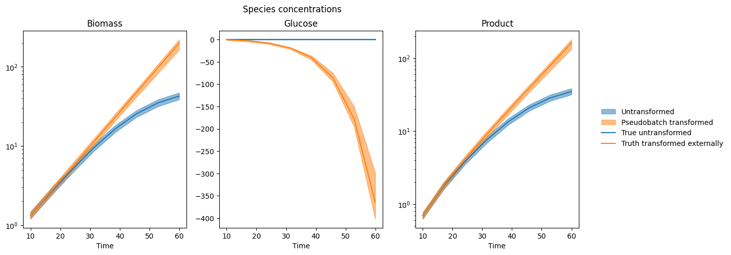
Plotting some modelled quantities

def plot_timecourse_qs(
    ax: plt.Axes,
    varname: str,
    idata_group: xr.Dataset,
    timepoints: pd.Series,
    coords: dict,
    quantiles: list = [0.025, 0.975],
    **fill_between_kwargs
) -> PolyCollection:
    var_draws = idata_group[varname]
    for k, v in coords.items():
        if k in var_draws.coords:
            var_draws = var_draws.sel({k:v})
    qs = var_draws.quantile(quantiles, dim=["chain", "draw"]).to_dataframe()[varname].unstack("quantile")
    low = qs[0.025].values
    high = qs[0.975].values
    x = timepoints.values
    return ax.fill_between(x, low, high, **fill_between_kwargs)


f, axes = plt.subplots(1, 3, figsize=[14, 5])
for ax, species in zip(axes, SPECIES):
    pcs = []
    line_patches = []
    for var, color in zip(["c", "pseudobatch_c"], ["tab:blue", "tab:orange"]):
        true_value_colname = "c_" + species if var == "c" else f"c_{species}_pseudobatch"
        pc = plot_timecourse_qs(
            ax,
            var,
            idata.posterior,
            samples["timestamp"],
            {"species": [species]},
            color=color,
            alpha=0.5,
        )
        pcs += [pc]
        line = ax.plot(samples["timestamp"], samples[true_value_colname], color=color)
        line_patches += [line[-1]]
    txt = ax.set(xlabel="Time", title=species)
    if all(samples[true_value_colname] > 0):
        ax.semilogy()

f.suptitle("Species concentrations")
legend = f.legend(
    [*pcs, *line_patches],
    ["Untransformed", "Pseudobatch transformed", "True untransformed", "Truth transformed externally"],
    ncol=1,
    loc="right",
    frameon=False,
    bbox_to_anchor = [1.11, 0.5]
)

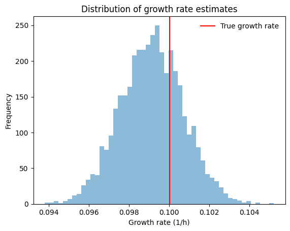
Estimating the growth rate

One thing that you might want to do with pseudobatch transformation is to estimate the measured cells’ growth rate.

This can be done for each sample from our posterior distribution, giving us an idea of the range of growth rate estimates that are consistent with our model. Even better, since we used a simulated dataset we know that the true growth rate is 0.1, so we can compare our estimated growth rates with the truth.

def fit_log_linear_model(y, x):
    logy = np.log(y.values)
    slope, intercept = np.polyfit(x, logy, deg=1)
    return xr.DataArray([slope, intercept])

growth_coeffs = pd.DataFrame(
    idata.posterior["pseudobatch_c"]
    .sel(species="Biomass")
    .stack(chaindraw=("chain", "draw"))
    .groupby("chaindraw")
    .map(fit_log_linear_model, x=samples["timestamp"], shortcut=True)
    .values,
    columns=["slope", "intercept"]
)
growth_coeffs.index.name = "draw"

display(growth_coeffs.T)

f, ax = plt.subplots()
hist = ax.hist(growth_coeffs["slope"], bins=50, alpha=0.5)
vline = ax.axvline(samples["mu_true"].iloc[0], c="red", label="True growth rate")
txt = ax.set(
    xlabel="Growth rate (1/h)",
    ylabel="Frequency",
    title="Distribution of growth rate estimates"
)
leg = ax.legend(frameon=False)


# the 0.025, 0.5 and 0.975 quantiles of the fitted slopes
# print(fitted_growth_rates.slope.quantile([0.025, 0.5, 0.975]))

draw	0	1	2	3	4	5	6	7	8	9	...	3990	3991	3992	3993	3994	3995	3996	3997	3998	3999
slope	0.102516	0.096615	0.101327	0.096538	0.101856	0.100044	0.099655	0.097026	0.099064	0.097570	...	0.101227	0.100904	0.099847	0.099308	0.099897	0.098900	0.099894	0.099580	0.10023	0.099364
intercept	-0.807900	-0.614030	-0.776267	-0.619113	-0.797399	-0.721281	-0.691591	-0.667151	-0.676970	-0.619378	...	-0.724136	-0.735155	-0.708653	-0.679298	-0.656992	-0.661648	-0.707765	-0.695189	-0.70449	-0.685411

2 rows × 4000 columns

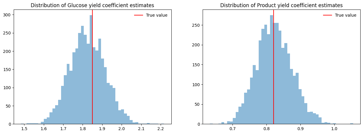
Estimating yield coefficients

def fit_linear_model(y, x):
    slope, intercept = np.polyfit(x, y, deg=1)
    return xr.DataArray([slope, intercept])

yield_dfs = {}

for species in ["Glucose", "Product"]:
    yield_dfs[species] = pd.DataFrame(
        idata.posterior["pseudobatch_c"]
        .sel(species=["Biomass", species])
        .stack(chaindraw=["chain", "draw"])
        .groupby("chaindraw")
        .map(lambda arr: fit_linear_model(arr.sel(species=species), arr.sel(species="Biomass")))
        .values,
        columns=["slope", "intercept"]
    )
print("Glucose yield coefficients:")
display(yield_dfs["Glucose"].T)
print("Product yield coefficients:")
display(yield_dfs["Product"].T)

f, axes = plt.subplots(1, 2, figsize=[15, 5])
for ax, species, true_value_colname in zip(axes, ["Glucose", "Product"], ["Yxs", "Yxp"]):
    hist = ax.hist(np.abs(yield_dfs[species]["slope"]), bins=50, alpha=0.5)
    vline = ax.axvline(samples[true_value_colname].iloc[0], color="red", label="True value")
    title = ax.set(title=f"Distribution of {species} yield coefficient estimates")
    leg = ax.legend(frameon=False)

Glucose yield coefficients:

	0	1	2	3	4	5	6	7	8	9	...	3990	3991	3992	3993	3994	3995	3996	3997	3998	3999
slope	-1.744210	-1.757008	-1.741915	-1.723624	-1.871941	-1.838772	-1.823377	-1.836021	-1.699397	-2.036570	...	-1.845025	-1.872864	-1.875026	-1.919493	-1.854989	-1.886462	-1.896649	-1.864343	-1.842283	-1.924881
intercept	-2.587623	1.628419	-0.189456	-0.116613	2.007992	2.594703	2.372684	0.084090	0.129974	4.094919	...	-1.764112	-1.661884	3.475286	4.223898	-0.092433	-1.238829	1.127363	1.162724	-0.245896	3.203416

2 rows × 4000 columns

Product yield coefficients:

	0	1	2	3	4	5	6	7	8	9	...	3990	3991	3992	3993	3994	3995	3996	3997	3998	3999
slope	0.717567	0.830149	0.799137	0.811471	0.820391	0.820898	0.781038	0.815743	0.803372	0.897239	...	0.833248	0.790404	0.889563	0.877858	0.808814	0.822912	0.862858	0.836267	0.825557	0.881137
intercept	2.035210	-0.845795	-0.920503	0.366229	-1.117119	-1.476975	-0.584068	0.767538	-0.163943	-1.097187	...	0.044753	1.346261	-2.497430	-2.395350	0.753787	0.738677	-0.983234	-1.065378	-0.643284	-1.157595

2 rows × 4000 columns