Special case: gaseous species

In this special case tutorial we will discuss how to handle gaseous compounds both in the in- and outlet of the reactor, the most common molecules of this type is CO2 and O2. We can setup the full mass balance for the gaseous species as follows:

\[\frac{dM_{species}}{dt}=In_{gas}+In_{liquid}-Out_{gas}+Metabolism-Sampled\]

where \(M_{species}\) is the total amount of species in the reactor in both gas and aqueous phase. The term metabolism is the net value and covers both production (positive) and consumption (negative). If we integrate the mass balance we get the following:

\[M_{species}(t)=\int_0^t In_{gas}+\int_0^t In_{liquid}-\int_0^t Out_{gas}+\int_0^t Metabolism-\int_0^t Sampled\]

This shows that the concentration of the species at a give time is result of the integrated mass balance, i.e. the accumulated “events”, e.g. input of medium, gas, sampling etc. We are interested in how the cells contribute to the changes in mass of the species, thus we will isolate the metabolism term.

\[\int_0^t Metabolism=M_{species}(t)-\int_0^t In_{gas}-\int_0^t In_{liquid}+\int_0^t Out_{gas}+\int_0^t Sampled\]

The mass balance above works in mass units, however, the pseudo batch transformation can only work with concentrations. Therefore, we treat the integrated metabolism as entirely solubilized and assign it a “hypothetical concentration”, which we then perform the pseudobatch correction on.

The pseudobatch package presents two functions which aids tranformation of gaseous species. The first calculates the hypothetical concentration from metabolism time series. The second function can calculate the metabolism term in the mass balance from the data.

In this tutorial we will go through three examples

1. Highly insoluble produced compound, exemplified by \(CO_2\)

2. Consumed gaseous compound, exemplified by \(O_2\)

3. Partially insoluble compound, exemplified by a generic product

Now, we are ready to setup the programming environment and load the data.

import matplotlib.pyplot as plt
import pandas as pd
import numpy as np

from pseudobatch import pseudobatch_transform_pandas, hypothetical_concentration, metabolised_amount
from pseudobatch.datasets import load_volatile_compounds_fedbatch

/Users/s143838/.virtualenvs/pseudobatch-dev/lib/python3.10/site-packages/tqdm/auto.py:21: TqdmWarning: IProgress not found. Please update jupyter and ipywidgets. See https://ipywidgets.readthedocs.io/en/stable/user_install.html
  from .autonotebook import tqdm as notebook_tqdm

{'stan_version_major': '2', 'stan_version_minor': '29', 'stan_version_patch': '2', 'STAN_THREADS': 'false', 'STAN_MPI': 'false', 'STAN_OPENCL': 'false', 'STAN_NO_RANGE_CHECKS': 'false', 'STAN_CPP_OPTIMS': 'false'}

fedbatch_df = load_volatile_compounds_fedbatch()

Transforming a highly insoluble produced compound, \(CO_2\)

When a compound is highly insoluble one can make a simplifying assumption, i.e. that all the product which is product exists the reactor through the off gas. Furthermore, we assume that there is no \(CO_2\) present in the inlet gas. If we look at the mass balance this assumption has the following effect.

\[\int_0^t Metabolism=\sout{M_{species}(t)}-\sout{\int_0^t In_{gas}}-\sout{\int_0^t In_{liquid}}+\int_0^t Out_{gas}+\sout{\int_0^t Sampled}\]

Thus, under these two assumptions all \(\int_0^t Metabolism=\int_0^t Out_{gas}\).

These two assumptions are true for the simulated test dataset. The data contain simulated the accumulated \(CO_2\) production measurements in mass units in the column m_CO2_gas. We can start by looking at the simulated \(CO_2\) data.

fedbatch_df.plot(x='timestamp', y=['c_CO2', 'm_CO2_gas'], subplots=True, layout=(2,1), label=['Aqueous concentration CO2 [g/L]', 'Accum. CO2 measured in gas [g]'])

array([[<Axes: xlabel='timestamp'>],
       [<Axes: xlabel='timestamp'>]], dtype=object)

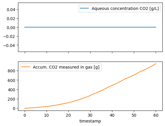
In the upper panel, we verify that \(CO_2\) does not accumulated in the medium. In the lower panel we see how the production rate of CO2 (g/h) decrease the bioreactor is sampled. This is because the total amount of biomass decrease after sampling, thus there is less biomass to produce CO2.

We assume that all \(CO_2\) that exists the bioreactor is product of metabolism, i.e. no \(CO_2\) is added through the liquid or gas feed. Therefore, we can directly calculate the hypothetical concentration from the off-gas measurements.

fedbatch_df['hypothetical_c_CO2'] = hypothetical_concentration(
    metabolised_amount=fedbatch_df['m_CO2_gas'].to_numpy(),
    reactor_volume=fedbatch_df['v_Volume'].to_numpy(),
    sample_volume=fedbatch_df['sample_volume'].to_numpy()
)

Now, we can transform the hypothetical CO2 concentration and the biomass concentration measurements.

fedbatch_df[['pseudo_Biomass', 'pseudo_CO2']] = pseudobatch_transform_pandas(
    df=fedbatch_df,
    measured_concentration_colnames=["c_Biomass", "hypothetical_c_CO2"],
    reactor_volume_colname='v_Volume',
    accumulated_feed_colname='v_Feed_accum',
    concentration_in_feed=[0,0],
    sample_volume_colname='sample_volume'
)

If we estimate the CO2 yield using the pseudobatch transformed data we obtain the exact value used for the simulation.

Yxco2_hat, intercept = np.polyfit(fedbatch_df['pseudo_Biomass'], fedbatch_df['pseudo_CO2'], 1)
print(f"Yxco2_hat = {Yxco2_hat}")
print(f"true Yxco2 = {fedbatch_df['Yxco2'].iloc[-1]}")

Yxco2_hat = 0.045193332445214125
true Yxco2 = 0.0451933324452141

Consumed gaseous species, Oxygen

The amount of metabolised \(O_2\) has to be calculated from the mass balance. When the oxygen enters the bioreactor some will go straight through and into the off-gas analyzer, and some will be solubilized in the aqueous phase. From the aqueous phase the \(O_2\) can either be metabolised or removed through sampling (or evaporate again). Thus, we need to solve the mass balance to find the amount of metabolised \(O_2\).

\[\int_0^t Metabolism=M_{species}(t)-\int_0^t In_{gas}-\int_0^t In_{liquid}+\int_0^t Out_{gas}+\int_0^t Sampled\]

Some of these terms are obtained from measurements and some can be estimated, e.g. the oxygen content in the liquid feed medium is rarely measured, but is likely insignificant. In this example, we will assume that \(\int_0^t In_{liquid}=0\) for all \(t\).

You can calculate the metabolized amount of \(O_2\) on your own, but it does require special care to use the correct volume and mass’ regarding before or after sampling. To ease the processes we have made a function which calculates the metabolized amount for you, metabolised_amount().

At the sampling time points this dataset contains the values just before the sample was taken. However, the metabolised_amount() function requires the values from just after the sample withdrawal. In the following we calculate the \(O_2\) mass after sample withdrawal.

fedbatch_df['m_O2_after_sample'] = fedbatch_df['m_O2'] - fedbatch_df['c_O2'] * fedbatch_df['sample_volume']

Here, we will use the metabolised_amount() function to calculate the mass of consumed \(O_2\).

fedbatch_df['m_O2_consumed'] = metabolised_amount(
    off_gas_amount=fedbatch_df['m_O2_gas'].to_numpy(),
    dissolved_amount_after_sampling=fedbatch_df['m_O2_after_sample'].to_numpy(),
    inlet_gas_amount=fedbatch_df['m_O2_in'].to_numpy(),
    sampled_amount=(fedbatch_df['c_O2'] * fedbatch_df['sample_volume']).cumsum().to_numpy(),
    inlet_liquid_amount=np.zeros_like(fedbatch_df['m_O2_in'].to_numpy()),
)

Now, that we have calculated the metabolised amount of \(O_2\) we can calculate the hypothetical concentration and run the pseudo batch transformation on the hypothetical concentration data.

fedbatch_df['hypothetical_c_O2'] = hypothetical_concentration(
    metabolised_amount=fedbatch_df['m_O2_consumed'].to_numpy(),
    reactor_volume=fedbatch_df['v_Volume'].to_numpy(),
    sample_volume=fedbatch_df['sample_volume'].to_numpy(),
)

fedbatch_df['pseudo_O2'] = pseudobatch_transform_pandas(
    df=fedbatch_df,
    measured_concentration_colnames=['hypothetical_c_O2'],
    reactor_volume_colname='v_Volume',
    accumulated_feed_colname='v_Feed_accum',
    concentration_in_feed=[0],
    sample_volume_colname='sample_volume',
)

We are now ready to estimate the oxygen yield coefficient using a linear model.

Yxo2_hat, intercept = np.polyfit(fedbatch_df['pseudo_Biomass'], fedbatch_df['pseudo_O2'], 1)
print(f"Yxo2_hat = {Yxo2_hat}")
print(f"true Yxo2 = {fedbatch_df['Yxo2'].iloc[-1]}")

Yxo2_hat = -0.010000000000000162
true Yxo2 = 0.01

We see that the estimated oxygen yield coefficient match the one used for simulating the data show the the method works.

Volatile product

Finally, we simulated a generic volatile product which is produced in the liquid and then evaporates through first order kinetics. We will assume that we have measurements both of the evaporating amount and the liquid concentration of the product. For the mass balance we will assume that both \(\int_0^t In_{gas}=0\) and \(\int_0^t In_{liquid}=0\).

Let’s first inspect the raw simulated data.

fedbatch_df.plot(
    x='timestamp',
    y=['m_Product', 'm_product_gas']
)

<Axes: xlabel='timestamp'>

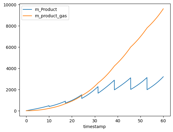
Some of the dissolved product (m_Product) is removed when the bioreactor is sampled, while the product that has evaporated is not removed through sampling. We need to calculate the total production of the product, i.e. combining the two curves above. We can use the metabolised_amount() to calculated the total production.

# again first we need to calculate the mass of product after sampling
# to obey the requirements of the metabolised_amount function
fedbatch_df['m_Product_after_sample'] = fedbatch_df['m_Product'].to_numpy() - (fedbatch_df['c_Product'] * fedbatch_df['sample_volume']).to_numpy()

fedbatch_df['m_Product_produced'] = metabolised_amount(
    off_gas_amount=fedbatch_df['m_product_gas'].to_numpy(),
    dissolved_amount_after_sampling=fedbatch_df['m_Product_after_sample'].to_numpy(),
    inlet_gas_amount=np.zeros_like(fedbatch_df['m_Product']),
    sampled_amount=(fedbatch_df['c_Product'] * fedbatch_df['sample_volume']).cumsum().to_numpy(),
)
fedbatch_df['hypothetical_c_Product'] = hypothetical_concentration(
    metabolised_amount=fedbatch_df['m_Product_produced'].to_numpy(),
    reactor_volume=fedbatch_df['v_Volume'].to_numpy(),
    sample_volume=fedbatch_df['sample_volume'].to_numpy()
)

Now that we have the hypothetical concentration we can perform pseudobatch transformation on the data.

fedbatch_df['pseudo_Product'] = pseudobatch_transform_pandas(
    df=fedbatch_df,
    measured_concentration_colnames='hypothetical_c_Product',
    reactor_volume_colname='v_Volume',
    accumulated_feed_colname='v_Feed_accum',
    concentration_in_feed=[0],
    sample_volume_colname='sample_volume'
)

Finally, we can estimate the product yield coefficient using a linear model.

Yxp_hat, intercept = np.polyfit(fedbatch_df['pseudo_Biomass'], fedbatch_df['pseudo_Product'], 1)
print(f"Yxp_hat = {Yxp_hat}")
print(f"true Yxp = {fedbatch_df['Yxp'].iloc[-1]}")

Yxp_hat = 0.8215102466751055
true Yxp = 0.8215102466751038

Again, we show that the estimated yield coefficient matches the coefficient that was used for the simulation.

Through out this tutorial we have shown that pseudobatch transformation is capable of handling measurements of gaseous compounds. And how to use the two helper functions hypethetical_concentration and metabolised_amount to prepare the measurements for pseudo batch transformation.