Pre-processing of LC-MS/MS metabolomics data using pyOpenMS

import os
import re

import matplotlib.pyplot as plt
import numpy as np
import pandas as pd
import pyopenms as oms

The relevant files are selected:

metadata = pd.read_csv("data/MTBLS8735/metadata.csv")

input_labels = metadata["phenotype"].tolist()

input_files = []
for i in range(len(metadata)):
    f = re.sub(r"FILES/", "", metadata["derived_spectra_data_file"][i])
    input_files.append("data/MTBLS8735/" + f)

fname_intern_standard = os.path.join("data", "MTBLS8735", "intern_standard_list.txt")

Data visualization

Before starting the pre-processing workflow, we visualize the Base Peak Chromatogram (BPC) for each sample. The BPC represents the intensity of the most intense ion detected in every MS1 spectrum over the course of the chromatographic run. Plotting the BPC provides a quick overview of the data quality and allows us to compare the overall signal profiles between samples. Similar chromatographic patterns across runs suggest consistent instrument performance, while large differences may indicate potential issues that should be investigated before proceeding with further analysis.

Show code cell source

Hide code cell source

def extract_bpc(exp):

    bpc_rt = []
    bpc_int = []

    for spec in exp:
        if spec.getMSLevel() != 1:
            continue

        peaks = spec.get_peaks()[1]  # intensities
        bpc_rt.append(spec.getRT())
        bpc_int.append(peaks.max() if len(peaks) else 0)
    return bpc_rt, bpc_int


colors = [
    "coral",
    "steelblue",
    "orchid",
    "coral",
    "orchid",
    "steelblue",
    "coral",
    "orchid",
    "steelblue",
    "coral",
]
for file, color, label in zip(input_files, colors, input_labels):
    exp = oms.MSExperiment()
    oms.MzMLFile().load(file, exp)
    rt, inten = extract_bpc(exp)
    plt.plot(rt, inten, color=color, alpha=0.5, lw=1.5, label=label)

plt.legend()
plt.grid()
plt.title("BPC")
plt.xlabel("Retention Time (s)")
plt.ylabel("Intensity")
plt.show()

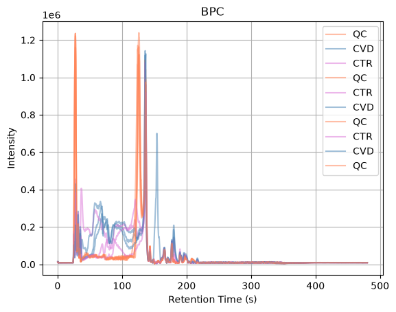
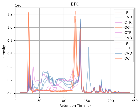
The BPC profiles show that the final portion of the chromatographic run contains little to no signal, indicating that no relevant compounds are being detected in this region. To reduce unnecessary data and focus the analysis on the informative part of the chromatogram, we filter the experiment by retention time and retain only spectra acquired between 10 and 240 seconds. The filtered BPCs allow us to verify that the useful chromatographic region has been preserved while removing empty sections that would otherwise increase processing time and data size.

Show code cell source

Hide code cell source

def filter_chr(file):
    filtered = oms.MSExperiment()
    exp = oms.MSExperiment()
    oms.MzMLFile().load(file, exp)

    for spec in exp:
        rt = spec.getRT()
        if 10 <= rt <= 240:
            filtered.addSpectrum(spec)

    return filtered


filtered_exps = []
for file in input_files:
    filtered = filter_chr(file)
    filtered_exps.append(filtered)

for exp, color, label in zip(filtered_exps, colors, input_labels):
    rt, inten = extract_bpc(exp)
    plt.plot(rt, inten, color=color, alpha=0.5, lw=1.5, label=label)

plt.legend()
plt.grid()
plt.title("BPC")
plt.xlabel("Retention Time (s)")
plt.ylabel("Intensity")
plt.show()

Next, we load a table containing a list of internal standards (IS). Internal standards are compounds with known properties that are often included in metabolomics experiments as reference signals. In this workflow, we are not using them for quantitative correction, but simply visualizing their behavior across samples. This helps us inspect their chromatographic profiles and use them as a practical reference when selecting or adjusting preprocessing parameters.

intern_standard = pd.read_csv(
    fname_intern_standard,
    sep="\t",
)
intern_standard

	name	abbreviation	formula	POS	NEG	RT	data_set	sample	operator	version	quality_NEG	quality_POS	mz	mzmin	mzmax	rtmin	rtmax
carnitine_d3	Carnitine (D3)	carnitine_d3	164.1240	[M+H]+	NaN	61	2019_11_matrix_effect	serum	Mar Garcia-Aloy	2	3_bad	2_medium	165.131276	165.126276	165.136276	51	71
creatinine_methyl_d3	Creatinine (N-Methyl_D3)	creatinine_methyl_d3	116.0777	[M+H]+	[M-H]-	126	2019_11_matrix_effect	serum	Mar Garcia-Aloy	2	2_medium	2_medium	117.084976	117.079976	117.089976	116	136
glucose_d2	Glucose (6,6-D2)	glucose_d2	182.0759	[M+Na]+	[M+CHO2]-	166	2019_11_matrix_effect	serum	Mar Garcia-Aloy	2	1_good	2_medium	205.065120	205.060120	205.070120	156	176
alanine_13C_15N	L-Alanine (13C3, 99%; 15N, 99%)	alanine_13C_15N	93.0548	[M+H]+	[M-H]-	167	2019_11_matrix_effect	serum	Mar Garcia-Aloy	2	2_medium	1_good	94.062076	94.057076	94.067076	157	177
arginine_13C_15N	L-Arginine HCl (13C6, 99%; 15N4, 99%)	arginine_13C_15N	184.1199	[M+H]+	[M-H]-	183	2019_11_matrix_effect	serum	Mar Garcia-Aloy	2	0_perfect	0_perfect	185.127176	185.122176	185.132176	173	193
aspartic_13C_15N	L-Aspartic acid (13C4, 99%; 15N, 99%)	aspartic_13C_15N	138.0480	[M+H]+	[M-H]-	179	2019_11_matrix_effect	serum	Mar Garcia-Aloy	2	1_good	1_good	139.055276	139.050276	139.060276	169	189
cystine_13C_15N	L-Cystine (13C6, 99%; 15N2, 99%)	cystine_13C_15N	248.0380	[M+H]+	[M-H]-	209	2019_11_matrix_effect	serum	Mar Garcia-Aloy	2	0_perfect	0_perfect	249.045276	249.040276	249.050276	199	219
glutamic_13C_15N	L-Glutamic acid (13C5, 99%; 15N, 99%)	glutamic_13C_15N	153.0670	[M+H]+	[M-H]-	171	2019_11_matrix_effect	serum	Mar Garcia-Aloy	2	0_perfect	0_perfect	154.074276	154.069276	154.079276	161	181
glycine_13C_15N	Glycine (13C2, 99%; 15N, 99%)	glycine_13C_15N	78.0358	[M+H]+	NaN	168	2019_11_matrix_effect	serum	Mar Garcia-Aloy	2	3_bad	1_good	79.043076	79.038076	79.048076	158	178
histidine_13C_15N	L-Histidine HCl H2O (13C6; 15N3, 99%)	histidine_13C_15N	164.0807	[M+H]+	[M-H]-	185	2019_11_matrix_effect	serum	Mar Garcia-Aloy	2	0_perfect	0_perfect	165.087976	165.082976	165.092976	175	195
isoleucine_13C_15N	L-Isoleucine (13C6, 99%; 15N, 99%)	isoleucine_13C_15N	138.1118	[M+H]+	[M-H]-	154	2019_11_matrix_effect	serum	Mar Garcia-Aloy	2	2_medium	2_medium	139.119076	139.114076	139.124076	144	164
leucine_13C_15N	L-Leucine (13C6, 99%; 15N, 99%)	leucine_13C_15N	138.1118	[M+H]+	[M-H]-	151	2019_11_matrix_effect	serum	Mar Garcia-Aloy	2	2_medium	2_medium	139.119076	139.114076	139.124076	141	161
lysine_13C_15N	L-Lysine 2HCl (13C6, 99%; 15N2, 99%)	lysine_13C_15N	154.1197	[M+H]+	[M-H]-	184	2019_11_matrix_effect	serum	Mar Garcia-Aloy	2	1_good	0_perfect	155.126976	155.121976	155.131976	174	194
methionine_13C_15N	L-Methionine (13C5, 99%; 15N, 99%)	methionine_13C_15N	155.0649	[M+H]+	[M-H]-	161	2019_11_matrix_effect	serum	Mar Garcia-Aloy	2	1_good	1_good	156.072176	156.067176	156.077176	151	171
phenylalanine_13C_15N	L-Phenylalanine (13C9, 99%; 15N, 99%)	phenylalanine_13C_15N	175.1062	[M+H]+	[M-H]-	153	2019_11_matrix_effect	serum	Mar Garcia-Aloy	2	1_good	1_good	176.113476	176.108476	176.118476	143	163
proline_13C_15N	L-Proline (13C5, 99%; 15N, 99%)	proline_13C_15N	121.0771	[M+H]+	[M-H]-	167	2019_11_matrix_effect	serum	Mar Garcia-Aloy	2	1_good	1_good	122.084376	122.079376	122.089376	157	177
serine_13C_15N	L-Serine (13C3, 99%; 15N, 99%)	serine_13C_15N	109.0497	[M+H]+	[M-H]-	178	2019_11_matrix_effect	serum	Mar Garcia-Aloy	2	1_good	0_perfect	110.056976	110.051976	110.061976	168	188
threonine_13C_15N	L-Threonine (13C4, 99%; 15N, 99%)	threonine_13C_15N	124.0687	[M+H]+	[M-H]-	171	2019_11_matrix_effect	serum	Mar Garcia-Aloy	2	0_perfect	0_perfect	125.075976	125.070976	125.080976	161	181
tyrosine_13C_15N	L-Tyrosine (13C9, 99%; 15N, 99%)	tyrosine_13C_15N	191.1011	[M+H]+	[M-H]-	166	2019_11_matrix_effect	serum	Mar Garcia-Aloy	2	1_good	1_good	192.108376	192.103376	192.113376	156	176
valine_13C_15N	L-Valine (13C5, 99%; 15N, 99%)	valine_13C_15N	123.0928	[M+H]+	[M-H]-	164	2019_11_matrix_effect	serum	Mar Garcia-Aloy	2	1_good	1_good	124.100076	124.095076	124.105076	154	174

To inspect the internal standards in more detail, we extract and visualize their Extracted Ion Chromatograms (EICs). An EIC represents the intensity of ions within a specific m/z range over time, restricted here to a defined retention time window.

For each internal standard, we select its expected m/z and retention time boundaries from the metadata table, and then compute a signal per MS1 spectrum by summing the intensities of all peaks that fall within the selected m/z window. This produces a chromatographic trace that reflects the elution profile of that compound in each sample.

Plotting these EICs across runs allows us to visually check peak shape, retention time consistency, and signal presence, which helps guide the selection of appropriate preprocessing parameters such as chromatographic width or signal-to-noise ratio.

Show code cell source

Hide code cell source

def extract_eic(exp, mzmin, mzmax, rtmin, rtmax):
    rt_list = []
    intensity_list = []

    for spec in exp:
        if spec.getMSLevel() != 1:
            continue

        rt = spec.getRT()
        if not (rtmin <= rt <= rtmax):
            continue

        mz, intensity = spec.get_peaks()

        mask = (mz >= mzmin) & (mz <= mzmax)

        if np.any(mask):
            rt_list.append(rt)
            intensity_list.append(intensity[mask].sum())
        else:
            rt_list.append(rt)
            intensity_list.append(0)

    return np.array(rt_list), np.array(intensity_list)


i = 7
mzmin = intern_standard["mzmin"].tolist()[i]
mzmax = intern_standard["mzmax"].tolist()[i]
rtmin = intern_standard["rtmin"].tolist()[i]
rtmax = intern_standard["rtmax"].tolist()[i]

for exp, color, label in zip(filtered_exps, colors, input_labels):
    rt, inten = extract_eic(exp, mzmin, mzmax, rtmin, rtmax)
    plt.plot(rt, inten, color=color, alpha=0.5, lw=1.5, label=label)

plt.legend()
plt.grid()
plt.title(f"EIC for {intern_standard.iloc[i]['name']}")
plt.xlabel("Retention Time (s)")
plt.ylabel("Intensity")
plt.show()

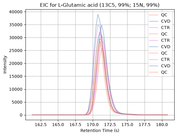
The different internal standards can be inspected by modifying the variable i. From the resulting EICs, we observe that internal standards 0, 1, 3, 10, 11, and 18 exhibit poor peak shapes or weak signal quality. We can also see that well-shaped peaks have a peak width of around 3-5 seconds.

Pre-processing - peak detection

We now perform peak detection, which is a three-step workflow that transforms raw MS1 data into a structured feature table.

First, Mass Trace Detection groups signals that share a similar m/z across consecutive scans, reconstructing continuous ion traces over retention time. Here, the parameter mass_error_ppm = 10.0 defines the allowed mass tolerance when grouping signals into the same trace. A relatively tight tolerance helps ensure that only signals with highly consistent m/z values are merged, improving trace specificity.

Second, Elution Peak Detection identifies true chromatographic peaks within each mass trace by evaluating their shape in the time domain. Several parameters control this step: chrom_peak_snr = 3.0 sets a minimum signal-to-noise threshold to reduce weak or noisy peaks, while chrom_fwhm = 3.0 defines the expected peak width (full width at half maximum) used to guide peak detection. This value is chosen based on the observed peak widths of well-behaved internal standards, which typically show widths of approximately 3–5 seconds. The bounds min_fwhm = 0.5 and max_fwhm = 5.0 further restrict acceptable peak widths based on this prior chromatographic behavior. Additionally, masstrace_snr_filtering = true enables filtering of low-quality mass traces before peak picking, improving robustness.

Finally, Feature Finding (Metabo) combines co-eluting mass traces into features that likely correspond to the same metabolite. The parameter charge_upper_bound = 1 restricts detection to singly charged ions, which is typical for many metabolomics datasets. chrom_fwhm = 3.0 again defines the expected chromatographic peak width used during grouping, while local_rt_range = chrom_fwhm * 2 sets the retention time window for associating signals across traces. isotope_filtering_model = none disables isotope pattern-based grouping, keeping the workflow simpler. Setting remove_single_traces = false ensures that features composed of only one mass trace are retained, and mz_scoring_by_elements = false disables element-based scoring of isotopic consistency. Finally, report_convex_hulls = true enables the storage of chromatographic boundaries, which can be useful for downstream visualization and inspection.

Show code cell source

Hide code cell source

rows = []
mass_traces_final_per_sample = []
features_per_sample = []
feature_maps = []

for s_idx, exp in enumerate(filtered_exps):

    mtd = oms.MassTraceDetection()
    params = mtd.getDefaults()

    params.setValue("mass_error_ppm", 10.0)
    mtd.setParameters(params)
    mass_traces = []
    mtd.run(exp, mass_traces, 0)

    mass_traces_split = []
    mass_traces_final = []
    epd = oms.ElutionPeakDetection()
    epd_params = epd.getDefaults()
    epd_params.setValue("width_filtering", "fixed")
    epd_params.setValue("chrom_peak_snr", 3.0)
    epd_params.setValue("chrom_fwhm", 3.0)
    epd_params.setValue("min_fwhm", 0.5)
    epd_params.setValue("max_fwhm", 7.0)
    epd_params.setValue("masstrace_snr_filtering", "true")
    epd.setParameters(epd_params)
    epd.detectPeaks(mass_traces, mass_traces_split)

    if epd.getParameters().getValue("width_filtering") == "auto":
        epd.filterByPeakWidth(mass_traces_split, mass_traces_final)
    else:
        mass_traces_final = mass_traces_split

    mass_traces_final_per_sample.append(len(mass_traces_final))

    fm = oms.FeatureMap()
    feat_chrom = []
    ffm = oms.FeatureFindingMetabo()
    ffm_params = ffm.getDefaults()
    ffm_params.setValue("charge_upper_bound", 1)
    ffm_params.setValue("chrom_fwhm", 3.0)
    ffm_params.setValue("local_rt_range", ffm_params.getValue("chrom_fwhm") * 2)
    ffm_params.setValue("isotope_filtering_model", "none")
    ffm_params.setValue(
        "remove_single_traces", "false"
    )  # set false to keep features with only one mass trace
    ffm_params.setValue("mz_scoring_by_elements", "false")
    ffm_params.setValue("report_convex_hulls", "true")
    # ffm_params.setValue("local_mz_range", 0.5)
    ffm.setParameters(ffm_params)
    ffm.run(mass_traces_final, fm, feat_chrom)

    fm.setUniqueIds()
    sample_name = os.path.basename(input_files[s_idx])
    print(sample_name)
    fm.setIdentifier(sample_name)
    fm.setPrimaryMSRunPath([sample_name.encode()])
    fm.setLoadedFilePath(input_files[s_idx])

    feature_maps.append(fm)

    peaklist = fm.get_df()

    features_per_sample.append(len(peaklist))

Progress of 'mass trace detection':
-- done [took 1.93 s (CPU), 1.91 s (Wall)] -- 
Progress of 'elution peak detection':
-- done [took 1.64 s (CPU), 0.43 s (Wall)] -- 
MS_QC_POOL_1_POS.mzML
Progress of 'assembling mass traces to features':
-- done [took 1.33 s (CPU), 0.38 s (Wall)] -- 
Progress of 'mass trace detection':
-- done [took 2.33 s (CPU), 2.31 s (Wall)] --
Progress of 'elution peak detection':
-- done [took 1.43 s (CPU), 0.37 s (Wall)] --
Progress of 'assembling mass traces to features':
-- done [took 1.14 s (CPU), 0.32 s (Wall)] -- 
MS_A_POS.mzML
Progress of 'mass trace detection':
-- done [took 2.13 s (CPU), 2.11 s (Wall)] -- 
Progress of 'elution peak detection':
-- done [took 1.41 s (CPU), 0.41 s (Wall)] -- 
Progress of 'assembling mass traces to features':
-- done [took 1.12 s (CPU), 0.31 s (Wall)] -- 
MS_B_POS.mzML
Progress of 'mass trace detection':
-- done [took 1.97 s (CPU), 1.96 s (Wall)] -- 
Progress of 'elution peak detection':
-- done [took 1.62 s (CPU), 0.43 s (Wall)] -- 
Progress of 'assembling mass traces to features':
-- done [took 1.29 s (CPU), 0.37 s (Wall)] -- 
MS_QC_POOL_2_POS.mzML
Progress of 'mass trace detection':
-- done [took 2.23 s (CPU), 2.21 s (Wall)] -- 
Progress of 'elution peak detection':
-- done [took 1.45 s (CPU), 0.38 s (Wall)] --
Progress of 'assembling mass traces to features':
-- done [took 1.11 s (CPU), 0.31 s (Wall)] -- 
MS_C_POS.mzML
Progress of 'mass trace detection':
-- done [took 2.30 s (CPU), 2.27 s (Wall)] --
MS_D_POS.mzMLProgress of 'elution peak detection':

-- done [took 1.47 s (CPU), 0.39 s (Wall)] -- 
Progress of 'assembling mass traces to features':
-- done [took 1.22 s (CPU), 0.34 s (Wall)] -- 
Progress of 'mass trace detection':
-- done [took 1.85 s (CPU), 1.84 s (Wall)] --
Progress of 'elution peak detection':
-- done [took 1.64 s (CPU), 0.43 s (Wall)] -- 
Progress of 'assembling mass traces to features':
-- done [took 1.28 s (CPU), 0.39 s (Wall)] -- 
MS_QC_POOL_3_POS.mzML
Progress of 'mass trace detection':
-- done [took 2.22 s (CPU), 2.20 s (Wall)] -- 
Progress of 'elution peak detection':
-- done [took 1.53 s (CPU), 0.40 s (Wall)] --
MS_E_POS.mzML
Progress of 'assembling mass traces to features':
-- done [took 1.31 s (CPU), 0.37 s (Wall)] --
Progress of 'mass trace detection':
-- done [took 2.39 s (CPU), 2.37 s (Wall)] -- 
Progress of 'elution peak detection':
-- done [took 1.43 s (CPU), 0.37 s (Wall)] -- 
MS_F_POS.mzML
Progress of 'assembling mass traces to features':
-- done [took 1.09 s (CPU), 0.30 s (Wall)] -- 
Progress of 'mass trace detection':
-- done [took 2.11 s (CPU), 2.09 s (Wall)] --
Progress of 'elution peak detection':
-- done [took 1.66 s (CPU), 0.44 s (Wall)] -- 
Progress of 'assembling mass traces to features':
-- done [took 1.32 s (CPU), 0.40 s (Wall)] -- 
MS_QC_POOL_4_POS.mzML

Show code cell source

Hide code cell source

for fm in feature_maps:
    print(fm.size())

15854
12719
13142
15752
13013
13124
15865
14736
12066
16289

And the peaklist:

peaklist

	peptide_sequence	peptide_score	ID_filename	ID_native_id	charge	rt	mz	rt_start	rt_end	mz_start	mz_end	quality	intensity
feature_id
7127830357663304158	None	NaN	None	None	0	190.000	50.015471	179.119	204.509	50.013222	50.018452	0.000003	143.119598
4763123553935025833	None	NaN	None	None	0	191.395	51.058931	190.558	196.696	51.058031	51.059849	0.000014	597.242554
8153770217427424435	None	NaN	None	None	0	205.904	51.941229	203.393	207.299	51.939158	51.943257	0.000002	104.045067
744891943546494316	None	NaN	None	None	0	202.835	51.986538	200.603	205.904	51.985807	51.987559	0.000009	403.690704
5452313450176978627	None	NaN	None	None	0	142.569	53.014043	141.453	146.196	53.012243	53.016863	0.000002	98.585320
...	...	...	...	...	...	...	...	...	...	...	...	...	...
10633491584310468569	None	NaN	None	None	0	60.820	999.889846	60.541	62.215	999.797537	999.963191	0.000001	58.130596
5685748652138019903	None	NaN	None	None	0	63.331	999.928486	62.773	69.190	999.809274	999.997863	0.000005	217.114456
4100824518074694947	None	NaN	None	None	0	56.635	999.928825	36.267	57.751	999.828429	1000.010724	0.000002	101.281685
17763072511834389701	None	NaN	None	None	0	70.585	999.941249	69.469	73.096	999.899695	1000.020110	0.000002	76.413040
5828258758398992156	None	NaN	None	None	0	59.425	999.944787	58.030	60.262	999.842352	999.990283	0.000002	106.489151

16289 rows × 13 columns

Pre-processing - peak alignment and matching

After feature detection, we perform retention time alignment and feature grouping to make features comparable across samples.

First, we select a reference feature map based on the sample with the highest number of detected features (fm.size()), under the assumption that it provides the most complete representation of the chromatographic signal. All other runs will be aligned to this reference.

We then apply the Pose Clustering Map Alignment algorithm, which corrects retention time shifts between samples by identifying corresponding feature patterns and estimating RT transformations. Each non-reference feature map is aligned individually, producing a transformation (TransformationDescription) that is then applied to adjust retention times using the MapAlignmentTransformer. This step ensures that the same compounds elute at comparable retention times across all runs.

Once alignment is completed, we construct a Consensus Map, which merges features across samples into a unified representation. This is achieved using the FeatureGroupingAlgorithmKD, which links features based on similarity in m/z and aligned retention time. The parameter warp:mz_tol = 15.0 defines the tolerated m/z deviation during grouping, while link:mz_tol = 15.0 controls the maximum m/z difference allowed when connecting features across runs. distance_MZ:exponent = 1.0 defines a linear weighting of m/z differences in the similarity scoring, and warp:max_nr_conflicts = 5 limits ambiguous assignments to improve grouping robustness.

The resulting consensus map contains a consolidated feature table, where each entry represents a putative metabolite observed across multiple samples, enabling downstream statistical analysis and annotation.

Show code cell source

Hide code cell source

ref_index = [
    i[0]
    for i in sorted(enumerate([fm.size() for fm in feature_maps]), key=lambda x: x[1])
][-1]
aligner = oms.MapAlignmentAlgorithmPoseClustering()
aligner.setReference(feature_maps[ref_index])

for i, fm in enumerate(feature_maps):

    if i == ref_index:
        continue

    trafo = oms.TransformationDescription()

    aligner.align(fm, trafo)

    transformer = oms.MapAlignmentTransformer()
    transformer.transformRetentionTimes(fm, trafo, True)

from pyopenms import ColumnHeader

consensus_map = oms.ConsensusMap()
file_descriptions = consensus_map.getColumnHeaders()

feature_grouper = (
    oms.FeatureGroupingAlgorithmKD()
)  # FeatureGroupingAlgorithmKD in metaboigniter
grouper_params = feature_grouper.getDefaults()
grouper_params.setValue("warp:mz_tol", 15.0)
grouper_params.setValue("link:mz_tol", 15.0)
grouper_params.setValue("distance_MZ:exponent", 1.0)
grouper_params.setValue("warp:max_nr_conflicts", 5)
feature_grouper.setParameters(grouper_params)

for i, feature_map in enumerate(feature_maps):
    file_description = file_descriptions.get(i, ColumnHeader())
    file_description.filename = feature_map.getMetaValue("spectra_data")[0].decode()
    file_description.size = feature_map.size()
    file_descriptions[i] = file_description

# execute feature linking:
feature_grouper.group(feature_maps, consensus_map)
consensus_map.setUniqueIds()
consensus_map.setColumnHeaders(file_descriptions)

print(f"Total number of consensus features: {consensus_map.size()}\n\n")

Progress of 'computing RT transformations':
-- done [took 0.96 s (CPU), 0.95 s (Wall)] -- 
Progress of 'linking features':
-- done [took 1.57 s (CPU), 1.56 s (Wall)] -- 
Total number of consensus features: 54872

peaklist = consensus_map.get_df()
sample_names = [os.path.basename(file) for file in input_files]
peaklist2 = peaklist[sample_names]

zero_counts = (peaklist2 == 0).sum(axis=1)

df_zeros = pd.DataFrame({"feature_id": peaklist2.index, "n_zeros": zero_counts})

freq_table = zero_counts.value_counts().sort_index()

df_freq = freq_table.reset_index()
df_freq.columns = ["Number_of_samples_with_0s", "n_features"]

df_freq

	Number_of_samples_with_0s	n_features
0	0	1772
1	1	1072
2	2	1136
3	3	1337
4	4	1743
5	5	2350
6	6	3460
7	7	4983
8	8	8729
9	9	28290

df = peaklist2.copy()
dict_0s = {}

for i in range(len(df)):
    n_0s = (df.iloc[i] == 0).sum()

    if n_0s not in dict_0s:
        dict_0s[n_0s] = []

    dict_0s[n_0s].append(i)

groups = list(dict_0s.keys())
samples = df.columns
result = pd.DataFrame(index=groups, columns=samples)

for j in samples:
    sample_is = df[j]
    for g in groups:
        sample_feats = sample_is.iloc[dict_0s[g]]
        n_0s = (sample_feats != 0).sum()
        result.loc[g, j] = n_0s

result

	MS_QC_POOL_1_POS.mzML	MS_A_POS.mzML	MS_B_POS.mzML	MS_QC_POOL_2_POS.mzML	MS_C_POS.mzML	MS_D_POS.mzML	MS_QC_POOL_3_POS.mzML	MS_E_POS.mzML	MS_F_POS.mzML	MS_QC_POOL_4_POS.mzML
0	1772	1772	1772	1772	1772	1772	1772	1772	1772	1772
1	971	952	975	975	933	973	985	990	912	982
2	919	890	944	939	840	915	935	924	853	929
3	924	903	947	938	873	974	959	991	865	985
4	1068	997	1070	1099	975	1061	1085	1075	951	1077
5	1274	1079	1081	1291	1047	1118	1271	1259	1040	1290
6	1675	1117	1202	1711	1189	1210	1704	1309	1052	1671
7	1807	1205	1310	1814	1235	1318	1819	1398	1135	1908
8	2058	1489	1470	2066	1487	1513	2091	1770	1337	2177
9	3386	2315	2371	3147	2662	2270	3244	3248	2149	3498

peaklist.to_csv("openms_peaklist.csv")