Metabolomics DSP Course - Data Analysis

In this demonstrative exercise, we will perform the downstream analysis of the Metabolights dataset MTBLS8735. This dataset contains three control samples derived from healthy samples, three samples from patients with Cardiovascular disease and four pooled Quality Control (QC) samples.

The rough workflow of this analysis is:

• Data filtering

• Imputation

• Correcting instrumental drift

• Normalisation and Visualisation

• Statistical analysis (ANCOVA)

For most of the analyses, we will be using the python package ACORE, which is a package developed by the Data Science Platform of NNF BRIGHT for analysing multi-omics molecular data - including metabolomics data. The documentation of this package can be found here: acore documentation. Go there to read about the functions in more detail, or to find out what else you can analyse with acore.

Although we are using acore for almost everything, all of these analyses can be carried out with other programs or in your own code, created in R, Python or other places, as well. This notebook serves primarily as a demonstration of the necessary steps of a typical downstream metabolomics data analysis.

Imports

import matplotlib.pyplot as plt
import matplotlib.transforms as transforms
import numpy as np
import pandas as pd
import vuecore.plots.basic.scatter
from matplotlib.patches import Ellipse
from sklearn.decomposition import PCA
from sklearn.preprocessing import StandardScaler

Helper functions

First, we are defining some helper functions. Feel free to ignore these while we go through the exercise, they are for example plotting functions. Do, however, run the cells.

Show code cell source

Hide code cell source

def plot_pca(
    df: pd.DataFrame,
    groups: dict[str, list],  # e.g. {"Control": [0,1,2], "Treatment": [3,4,5]}
    scale: bool = True,
    n_components: int = 2,
    figsize: tuple = (7, 5),
    title: str = "PCA Score Plot",
    palette: list = None,
    ellipse: bool = True,  # 95% confidence ellipse per group
    label_points: bool = False,  # annotate each point with its index
):
    """
    PCA score plot for metabolomics data.

    Parameters
    ----------
    df          : samples × features DataFrame (rows = samples)
    groups      : dict mapping group name -> list of row indices (int or label)
    scale       : z-score scale features before PCA (recommended)
    n_components: number of PCs to compute (≥2)
    ellipse     : draw a 95% confidence ellipse per group
    label_points: annotate each dot with its row index/label
    """

    # build ordered index and group label array
    all_idx = [i for idxs in groups.values() for i in idxs]
    group_labels = {i: grp for grp, idxs in groups.items() for i in idxs}

    X = df.loc[all_idx].copy()
    labels = [group_labels[i] for i in X.index]

    # scale & fit PCA
    if scale:
        X_vals = StandardScaler().fit_transform(X.values)
    else:
        X_vals = X.values

    pca = PCA(n_components=n_components)
    scores = pca.fit_transform(X_vals)
    var_exp = pca.explained_variance_ratio_ * 100

    # colours
    group_names = list(groups.keys())
    if palette is None:
        palette = plt.rcParams["axes.prop_cycle"].by_key()["color"]
    color_map = {g: palette[i % len(palette)] for i, g in enumerate(group_names)}

    # plot
    fig, ax = plt.subplots(figsize=figsize)

    for grp in group_names:
        mask = [l == grp for l in labels]
        pts = scores[mask]
        color = color_map[grp]

        ax.scatter(pts[:, 0], pts[:, 1], label=grp, color=color, s=80, zorder=3)

        if label_points:
            idx_list = groups[grp]
            for pt, idx in zip(pts, idx_list):
                ax.annotate(
                    str(idx), pt, textcoords="offset points", xytext=(5, 4), fontsize=8
                )

        if ellipse and len(pts) > 2:
            _confidence_ellipse(pts[:, 0], pts[:, 1], ax, color=color)

    ax.axhline(0, color="grey", lw=0.5, ls="--")
    ax.axvline(0, color="grey", lw=0.5, ls="--")
    ax.set_xlabel(f"PC1 ({var_exp[0]:.1f}%)", fontsize=12)
    ax.set_ylabel(f"PC2 ({var_exp[1]:.1f}%)", fontsize=12)
    ax.set_title(title, fontsize=13)
    ax.legend(framealpha=0.3)
    plt.tight_layout()
    plt.show()

    return pca, scores, var_exp


def _confidence_ellipse(x, y, ax, n_std=1.96, color="tab:blue", alpha=0.15, **kwargs):
    """Draw a covariance-based 95% confidence ellipse."""

    cov = np.cov(x, y)
    pearson = cov[0, 1] / np.sqrt(cov[0, 0] * cov[1, 1])
    rx = np.sqrt(1 + pearson)
    ry = np.sqrt(1 - pearson)

    ellipse = Ellipse(
        (0, 0),
        width=rx * 2,
        height=ry * 2,
        facecolor=color,
        alpha=alpha,
        edgecolor=color,
        linewidth=1.5,
        linestyle="--",
        **kwargs,
    )
    scale_x = np.sqrt(cov[0, 0]) * n_std
    scale_y = np.sqrt(cov[1, 1]) * n_std
    mean_x, mean_y = np.mean(x), np.mean(y)

    t = (
        transforms.Affine2D()
        .rotate_deg(45)
        .scale(scale_x, scale_y)
        .translate(mean_x, mean_y)
    )

    ellipse.set_transform(t + ax.transData)
    ax.add_patch(ellipse)


def plot_feature_missingness(data):
    missing_features = data.isnull().mean() * 100
    missing_features_nonzero = missing_features[missing_features > 0]

    fig, axes = plt.subplots(1, 2, figsize=(14, 5))

    # Histogram
    ax = axes[0]
    ax.hist(
        missing_features_nonzero.values,
        bins=30,
        color="mediumvioletred",
        edgecolor="white",
        linewidth=0.5,
    )
    ax.set_xlabel("Missing (%)")
    ax.set_ylabel("Number of features")
    ax.set_title(
        f"Distribution of missingness\n({len(missing_features_nonzero)} features with any missing)"
    )
    ax.axvline(
        x=20, color="black", linestyle="--", linewidth=0.8, label="20% threshold"
    )
    ax.legend()

    # Dot plot, sorted by missingness
    ax = axes[1]
    sorted_missing = missing_features.sort_values(ascending=True).reset_index(drop=True)
    ax.scatter(
        sorted_missing.index,
        sorted_missing.values,
        s=4,
        color="mediumvioletred",
        alpha=0.6,
        linewidths=0,
    )
    ax.set_xlabel("Features (sorted by missingness)")
    ax.set_ylabel("Missing (%)")
    ax.set_title("Sorted missingness per feature")
    ax.axhline(
        y=20, color="black", linestyle="--", linewidth=0.8, label="20% threshold"
    )
    ax.legend()

    plt.tight_layout()
    plt.show()


def missingness_summary(df_before, df_after):
    total = df_before.size
    n_before = df_before.isnull().sum().sum()
    n_after = df_after.isnull().sum().sum()

    print(f"Total values      : {total:,}")
    print(f"Missing before    : {n_before:,}  ({100*n_before/total:.1f}%)")
    print(f"Missing after     : {n_after:,}  ({100*n_after/total:.1f}%)")
    print(
        f"Features affected : {(df_before.isnull().any()).sum()} / {df_before.shape[1]}"
    )
    print(
        f"Samples affected  : {(df_before.isnull().any(axis=1)).sum()} / {df_before.shape[0]}"
    )


def plot_intensity_distribution(data):
    values = data.values.flatten().astype(float)

    n_total = data.size
    n_missing = int(np.isnan(values).sum())
    pct_missing = n_missing / n_total * 100

    log_values = np.log10(values[(~np.isnan(values)) & (values > 0)])

    fig, (ax_nan, ax_hist) = plt.subplots(
        1, 2, figsize=(11, 5), gridspec_kw={"width_ratios": [1, 8]}, sharey=True
    )

    ax_nan.bar(0, n_missing, width=0.2, color="mediumvioletred", alpha=0.8)
    ax_nan.set_xlim(-0.5, 0.5)
    ax_nan.set_xticks([0])
    ax_nan.set_xticklabels([f"NaN\n({pct_missing:.1f}%)"], fontsize=9)
    ax_nan.set_ylabel("Count")

    ax_hist.hist(
        log_values, bins=100, color="cornflowerblue", edgecolor="none", alpha=0.8
    )
    ax_hist.set_xlabel("Intensity (log₁₀)")
    ax_hist.set_title("Intensity distribution (all features, all samples)")
    ax_hist.yaxis.set_visible(False)

    plt.tight_layout()
    plt.show()


def plot_loess_example_curve(
    df: pd.DataFrame,
    feature_idx: int,
    samples: list,
    qcs: list,
    sample_order: pd.DataFrame,
    show_corrected: bool = True,
    alpha: float = None,  # fixed smoothing span; if None, selected by LOOCV
):
    """
    Plot the raw intensities, LOESS drift curve, and optionally the corrected
    intensities for a single feature according to the loess drift correction function.
    Useful for inspecting drift behaviour before running full drift correction.

    The drift curve is estimated with the same method used by
    ldc.run_drift_correction: LOESS is fit to the QC points and then
    interpolated across all injection positions via a cubic spline
    (qc_rlsc_loess).

    Parameters
    ----------
    df : pd.DataFrame
        Feature matrix with samples as rows and features as columns.
        Metadata columns should have been removed already.
    feature_idx : int
        Column index of the feature to plot.
    samples : list of str
        Row index labels of the biological samples.
    qcs : list of str
        Row index labels of the pooled QC samples.
    sample_order : pd.DataFrame
        Injection-order table with columns `File Name` and `Sample ID`
        (integer run order).
    show_corrected : bool, optional
        If True (default), overlays drift-corrected sample intensities as
        diamond markers.
    alpha : float, optional
        LOESS smoothing span (0 < α ≤ 1). If None (default), the optimal span
        is selected automatically by leave-one-out cross-validation over
        α ∈ [0.40, 1.00]. The selected value is shown in the legend.
    """

    all_rows = samples + qcs
    feature_col = df.iloc[:, feature_idx]

    order_dict = sample_order.set_index("File Name")["Sample ID"].to_dict()
    x_all = np.array([order_dict.get(r, np.nan) for r in all_rows])
    y_all = feature_col.loc[all_rows].astype(float).values

    n_s = len(samples)
    x_sample, y_sample = x_all[:n_s], y_all[:n_s]
    x_qc_arr, y_qc_arr = x_all[n_s:], y_all[n_s:]

    valid_sample = ~np.isnan(x_sample) & ~np.isnan(y_sample)
    valid_qc = ~np.isnan(x_qc_arr) & ~np.isnan(y_qc_arr)
    x_s_v, y_s_v = x_sample[valid_sample], y_sample[valid_sample]
    x_qc_v, y_qc_v = x_qc_arr[valid_qc], y_qc_arr[valid_qc]

    feature_name = df.columns[feature_idx]

    fig, ax = plt.subplots(figsize=(11, 5))
    ax.scatter(x_s_v, y_s_v, label="Samples", color="steelblue", alpha=0.7, zorder=3)
    ax.scatter(
        x_qc_v, y_qc_v, label="QC", color="firebrick", edgecolor="k", s=60, zorder=4
    )

    if len(x_qc_v) >= 4:
        if alpha is not None:
            # Pass a single-element candidate list to skip LOOCV and use the given alpha
            # directly
            drift_curve, best_alpha = dc.qc_rlsc_loess(
                x_qc_v, y_qc_v, x_all, always_use_default=True, default=alpha
            )
        else:
            drift_curve, best_alpha = dc.qc_rlsc_loess(x_qc_v, y_qc_v, x_all)

        valid_curve = ~np.isnan(x_all) & ~np.isnan(drift_curve)
        sort_idx = np.argsort(x_all[valid_curve])
        ax.plot(
            x_all[valid_curve][sort_idx],
            drift_curve[valid_curve][sort_idx],
            label=f"LOESS drift curve (α={best_alpha:.2f})",
            color="black",
            lw=2,
            zorder=5,
        )

        if show_corrected:
            median_qc = np.median(y_qc_v)
            drift_at_samples = drift_curve[:n_s][valid_sample]
            corrected = (y_s_v / drift_at_samples) * median_qc
            ax.scatter(
                x_s_v,
                corrected,
                label="Corrected samples",
                color="lightsteelblue",
                marker="D",
                s=40,
                alpha=0.9,
                zorder=3,
            )
    else:
        print(f"Not enough valid QC points for LOESS ({len(x_qc_v)} found, need ≥4).")

    ax.set_xlabel("Injection Order")
    ax.set_ylabel("Intensity")
    ax.set_title(f"Drift correction example ({feature_name})")
    ax.legend()
    ax.grid(True, alpha=0.3)
    plt.tight_layout()
    plt.show()


def pca_for_cpca_drift(
    df: pd.DataFrame,
    samples,  # list of row index labels, OR dict {group_name: [row index labels]}
    qcs: list,
    log_transform: bool = True,
    title: str = "PCA",
):
    """
    PCA of samples and QC samples.

    Parameters
    ----------
    df      : feature matrix with samples as rows and features as columns.
              Metadata columns should have been removed already.
    samples : list of row index labels of the biological samples (all one group),
              or dict {group_name: [row index labels]} for multiple groups
    qcs     : list of row index labels of the pooled QC samples
    log_transform : apply log1p before scaling
    title   : plot title
    """
    # Normalise samples to a dict
    if isinstance(samples, list):
        sample_groups = {"Samples": samples}
    else:
        sample_groups = samples

    # Build ordered row + label arrays
    all_rows, labels = [], []
    for group, rows in sample_groups.items():
        for r in rows:
            if r in df.index:
                all_rows.append(r)
                labels.append(group)
    for r in qcs:
        if r in df.index:
            all_rows.append(r)
            labels.append("QC")

    # Coerce to numeric, drop features (columns) with any NaN
    X = df.loc[all_rows].apply(pd.to_numeric, errors="coerce").dropna(axis=1)

    if log_transform:
        X = np.log1p(X.clip(lower=0))

    X_scaled = StandardScaler().fit_transform(X.values.astype(float))

    pca = PCA(n_components=2)
    coords = pca.fit_transform(X_scaled)
    pc1_var = pca.explained_variance_ratio_[0] * 100
    pc2_var = pca.explained_variance_ratio_[1] * 100

    palette = plt.cm.tab10.colors
    color_map = {g: palette[i % len(palette)] for i, g in enumerate(sample_groups)}
    color_map["QC"] = "black"

    fig, ax = plt.subplots(figsize=(8, 6))
    for group in list(sample_groups) + ["QC"]:
        mask = [_label == group for _label in labels]
        pts = coords[mask]
        is_qc = group == "QC"
        ax.scatter(
            pts[:, 0],
            pts[:, 1],
            label=group,
            color=color_map[group],
            marker="D" if is_qc else "o",
            s=70 if is_qc else 50,
            edgecolors="k" if is_qc else "none",
            alpha=0.9 if is_qc else 0.75,
            zorder=5 if is_qc else 3,
        )

    ax.set_xlabel(f"PC1 ({pc1_var:.1f}%)")
    ax.set_ylabel(f"PC2 ({pc2_var:.1f}%)")
    ax.set_title(title)
    ax.axhline(0, color="grey", lw=0.5, ls="--")
    ax.axvline(0, color="grey", lw=0.5, ls="--")
    ax.legend(framealpha=0.8)
    ax.grid(True, alpha=0.2)
    plt.tight_layout()
    plt.show()

Data setup

fname_features = "results_prepared/output_quantification_Linked_data.tsv"
fname_metadata = "data/MTBLS8735/metadata.csv"

First, let’s load and have a look at our data. You can find it in the data folder of this codespace.

metaboigniter_data = pd.read_csv(
    fname_features,
    sep="\t",
    index_col=0,
    dtype={"id": str},
)
metaboigniter_data

	charge	RT	mz	quality	MS_D_POS.mzML	MS_C_POS.mzML	MS_E_POS.mzML	MS_B_POS.mzML	MS_A_POS.mzML	MS_QC_POOL_1_POS.mzML	MS_QC_POOL_4_POS.mzML	MS_QC_POOL_3_POS.mzML	MS_F_POS.mzML	MS_QC_POOL_2_POS.mzML	adduct	feature_ids
id
1785900975374656749	0	82.991657	487.360409	0.000045	2197.7150	2499.92530	2055.4453	1789.1910	1737.8285	2228.8013	1863.83950	2093.6409	1761.39360	1882.0083	NaN	[10439623260835028, 1044712869837677293, 82553...
10359796054321139656	0	145.385393	141.958245	0.000026	1745.7393	987.70935	1540.5591	1862.1211	826.2672	555.4885	642.15070	1176.8750	997.84753	1006.0284	[M+H]+	[31491152637877450, 16826451592456168833, 8068...
17114916068296246246	1	203.540336	151.035251	0.000984	43793.8500	42707.09000	44408.4000	35033.9800	47008.1200	31749.9700	31151.19000	33077.8100	42819.70000	33124.9000	[M+H]+	[121786566209455346, 16662184219603302854, 103...
10875454315052802400	1	182.913495	342.015418	0.000209	14125.5400	11501.71000	9088.2600	6860.9673	12174.5300	1247.7310	2869.22780	2894.0437	12748.26000	4556.0920	[M+H]+	[130187692158764043, 8708957191126143269, 5655...
15167360593113340842	1	111.636771	491.300119	0.004628	143542.6000	173214.20000	89948.0100	93468.9200	157576.2000	198321.3000	207862.40000	206423.1000	169903.50000	204664.5000	[M+H]+	[163715205785070798, 15732231754378009136, 181...
...	...	...	...	...	...	...	...	...	...	...	...	...	...	...	...	...
17892945075043156858	0	125.446453	447.290728	0.000025	0.0000	0.00000	0.0000	0.0000	0.0000	0.0000	1229.67710	0.0000	0.00000	0.0000	NaN	[18165040187458211252]
2906889230784610727	0	33.937876	560.274926	0.000014	0.0000	0.00000	0.0000	0.0000	0.0000	0.0000	679.27590	0.0000	0.00000	0.0000	NaN	[18167075448252607803]
17135030643150808614	0	40.633406	341.263868	0.000013	0.0000	0.00000	0.0000	0.0000	0.0000	0.0000	659.15150	0.0000	0.00000	0.0000	NaN	[18283503193542699509]
2244705787916254982	0	33.937876	578.342658	0.000022	0.0000	0.00000	0.0000	0.0000	0.0000	0.0000	1072.48970	0.0000	0.00000	0.0000	NaN	[18283940505064136015]
10873393075126387345	0	35.611759	676.320660	0.000014	0.0000	0.00000	0.0000	0.0000	0.0000	0.0000	698.24835	0.0000	0.00000	0.0000	NaN	[18291256843486362483]

13094 rows × 16 columns

metaboigniter_data.columns

Index(['charge', 'RT', 'mz', 'quality', 'MS_D_POS.mzML', 'MS_C_POS.mzML',
       'MS_E_POS.mzML', 'MS_B_POS.mzML', 'MS_A_POS.mzML',
       'MS_QC_POOL_1_POS.mzML', 'MS_QC_POOL_4_POS.mzML',
       'MS_QC_POOL_3_POS.mzML', 'MS_F_POS.mzML', 'MS_QC_POOL_2_POS.mzML',
       'adduct', 'feature_ids'],
      dtype='object')

You can see that we have our features in the rows, and that there are 9068 of them. We have some metadata like mass-to-charge ratios and retention times, and then we have our intensities.

In order to properly analyse our data, we have to transpose it first. We also have to remove the metadata columns.

data = metaboigniter_data.T
data = data.drop(["charge", "RT", "mz", "quality", "adduct", "feature_ids"])
data = data.where(data > 1, np.nan)
data

id	1785900975374656749	10359796054321139656	17114916068296246246	10875454315052802400	15167360593113340842	7744533318583132094	1718920057707733684	6744901733644451055	11872048905895506999	13329452032929808115	...	3029767587063264539	17167452654274772591	8248272264971643600	3480066978786852155	17040961437395340439	17892945075043156858	2906889230784610727	17135030643150808614	2244705787916254982	10873393075126387345
MS_D_POS.mzML	2197.715	1745.7393	43793.85	14125.54	143542.6	1585.027	7369.8022	5886.109	11476.87	3449.8782	...	NaN	NaN	NaN	NaN	NaN	NaN	NaN	NaN	NaN	NaN
MS_C_POS.mzML	2499.9253	987.70935	42707.09	11501.71	173214.2	1210.8177	5918.5693	4802.169	10514.19	2679.616	...	NaN	NaN	NaN	NaN	NaN	NaN	NaN	NaN	NaN	NaN
MS_E_POS.mzML	2055.4453	1540.5591	44408.4	9088.26	89948.01	4690.5874	6250.251	5141.211	10575.09	2356.0645	...	NaN	NaN	NaN	NaN	NaN	NaN	NaN	NaN	NaN	NaN
MS_B_POS.mzML	1789.191	1862.1211	35033.98	6860.9673	93468.92	5135.8164	6641.842	2480.7393	8486.273	3797.3372	...	NaN	NaN	NaN	NaN	NaN	NaN	NaN	NaN	NaN	NaN
MS_A_POS.mzML	1737.8285	826.2672	47008.12	12174.53	157576.2	2573.8994	5735.305	6731.2915	9867.111	6096.421	...	NaN	NaN	NaN	NaN	NaN	NaN	NaN	NaN	NaN	NaN
MS_QC_POOL_1_POS.mzML	2228.8013	555.4885	31749.97	1247.731	198321.3	8646.111	8258.921	4336.047	9133.133	4147.0293	...	NaN	NaN	NaN	NaN	NaN	NaN	NaN	NaN	NaN	NaN
MS_QC_POOL_4_POS.mzML	1863.8395	642.1507	31151.19	2869.2278	207862.4	6730.96	9196.043	4037.6926	9277.422	4504.331	...	666.54095	2721.9639	1475.8854	954.4274	1300.5066	1229.6771	679.2759	659.1515	1072.4897	698.24835
MS_QC_POOL_3_POS.mzML	2093.6409	1176.875	33077.81	2894.0437	206423.1	8941.185	9147.992	4297.844	9498.344	5428.016	...	NaN	NaN	NaN	NaN	NaN	NaN	NaN	NaN	NaN	NaN
MS_F_POS.mzML	1761.3936	997.84753	42819.7	12748.26	169903.5	2100.4517	6168.7725	5676.127	10521.12	2820.938	...	NaN	NaN	NaN	NaN	NaN	NaN	NaN	NaN	NaN	NaN
MS_QC_POOL_2_POS.mzML	1882.0083	1006.0284	33124.9	4556.092	204664.5	7594.9097	7804.082	4517.161	9515.199	4617.7646	...	NaN	NaN	NaN	NaN	NaN	NaN	NaN	NaN	NaN	NaN

10 rows × 13094 columns

Now our data consists of only features in the columns, and samples in the rows.

We are also going to define some variables that help us later on in the code.

samples = [
    "MS_F_POS.mzML",
    "MS_E_POS.mzML",
    "MS_C_POS.mzML",
    "MS_A_POS.mzML",
    "MS_B_POS.mzML",
    "MS_D_POS.mzML",
]
samples_cvd = ["MS_F_POS.mzML", "MS_A_POS.mzML", "MS_D_POS.mzML"]
samples_ctr = ["MS_E_POS.mzML", "MS_C_POS.mzML", "MS_B_POS.mzML"]
qcs = [
    "MS_QC_POOL_1_POS.mzML",
    "MS_QC_POOL_2_POS.mzML",
    "MS_QC_POOL_3_POS.mzML",
    "MS_QC_POOL_4_POS.mzML",
]


groups_samples = {
    "CTR": samples_ctr,
    "CVD": samples_cvd,
}
groups_all = {
    "CTR": samples_ctr,
    "CVD": samples_cvd,
    "QC": qcs,
}

Data filtering

As a first step, we need to filter our data. There are many features in the data which are artifacts, background noise or unreliable. Additionally, there is a lot of missingness. While missing values can be imputed, it’s better to remove features with high levels of missingness first and only impute features that have signal in most samples.

We will use three methods of filtering:

• 80%-rule

• Coefficient of Variation (CV)-based filtering

• Dispersion ratio (D-ratio) filtering

For most of these, we will use the filter_metabolomics module from acore.

from acore import filter_metabolomics as fm

Let’s first check how much missingness there is in the data.

data.isna().sum().sum()
missing_per_feature = data.isna().sum(axis=0)
missing_per_feature
freq_table = missing_per_feature.value_counts().sort_index()

df_freq = freq_table.reset_index()
df_freq.columns = ["n_missing", "n_features"]

df_freq

	n_missing	n_features
0	0	1,084
1	1	369
2	2	314
3	3	383
4	4	491
5	5	577
6	6	985
7	7	1,106
8	8	1,801
9	9	5,984

plot_feature_missingness(data)
plot_intensity_distribution(data)

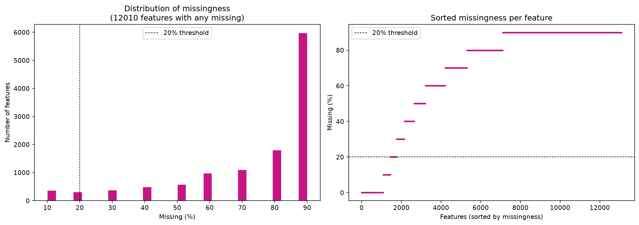
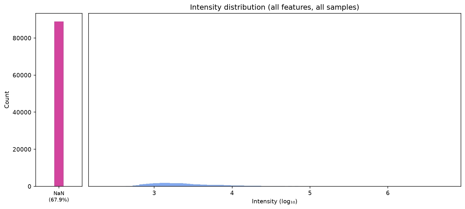
There are a lot of missing values, so it is important that we filter first.

80%-rule for filtering

The 80%-rule filters out features with too much missingness from our data. More specifically, if for a feature, more than 20% of the data is missing across all sample columns, it will be removed, so features must have at least 80% of data present in order to be retained.

Although it is called the 80%-rule, other thresholds can be used to make the filtering more lenient or more stringent.

In acore, this method is implemented in the function filter_by_missingness. Let’s first have a look at our function.

help(fm.filter_by_missingness)

Help on function filter_by_missingness in module acore.filter_metabolomics:

filter_by_missingness(data: pandas.core.frame.DataFrame, percent: int = 80, method: str = 'classic', samples: list | None = None, groups: dict | str | None = None)
    Implementation of the 80%-rule.

    If there are more than 20% of values (intensities) missing for one feature,
    this feature will get removed.

    :param data: pandas data frame with samples as rows and features as columns.
    :param percent: percentage chosen for filtering. The default is 80%, meaning that
        at least 80% of the values of every feature need to be present in order for this
        feature to be retained.
    :param method: str that is either "classic" or "modified".
        If "classic", all samples are considered for each feature. Samples are taken from the
        "samples" parameter and should not include controls or QCs.
        If "modified", conditions are separated when calculating the percentage of
        missingness. A feature is retained if at least ``percent``% of its values are
        present in ANY one condition. This allows condition-specific features (e.g.
        present in treatment but missing in control) to be retained.
    :param samples: list of row index labels (from data.index) identifying the biological
        sample rows, e.g. ["S1", "S2", "S3"]. Required when method="classic". Should not
        include control or QC samples.
    :param groups: required when method="modified", ignored otherwise. Can be either:

        - A dict mapping condition name to a list of row index labels belonging to that
          condition, e.g. ``{"treatment": ["S1", "S2", "S3"], "control": ["S4", "S5"]}``.
          QCs and blanks are excluded by simply not including them in the dict.
        - A str naming a column in ``data`` whose values define the condition for each row,
          e.g. ``"sample collection"`` if rows carry values like ``"Berlin"``, ``"Copenhagen"``, ``"London"``.
          Every unique value in that column becomes a condition group containing all rows
          with that value. When using this option, make sure to not include any other metadata
          columns in the data frame.

data_filtered_1 = fm.filter_by_missingness(
    data=data,
    method="classic",
    percent=80,  # 80% present, 20% missing is allowed at most
    samples=samples,
)

print(
    f"Num. of features before filtering: {data.shape[1]}\n"
    f"Num. of features after filtering: {data_filtered_1.shape[1]}"
)
print(f"Difference: {data.shape[1]-data_filtered_1.shape[1]} features removed.")

Num. of features before filtering: 13094
Num. of features after filtering: 2030
Difference: 11064 features removed.

missing_per_feature = data_filtered_1.isna().sum(axis=0)
freq_table = missing_per_feature.value_counts().sort_index()

df_freq = freq_table.reset_index()
df_freq.columns = ["n_missing", "n_features"]

df_freq

	n_missing	n_features
0	0	1,084
1	1	369
2	2	156
3	3	143
4	4	161
5	5	117

Now we have removed a huge number of features, and we have 2402 features left, which is a number we can trust more to contain real metabolites.

CV-based filtering

In this method, we are taking into account the quality control (QC) samples.

The CV of the biological samples and the CV of the QC samples are calculated per feature, and if for a given feature the CV of the QC samples is larger than that of the biological samples, it is removed. Also, if there are not enough QC samples to calculate the CV, or the mean is near zero, the features will be removed.

In acore, this method is implemented in the function filter_cv.

data_filtered_2 = fm.filter_cv(data=data_filtered_1, samples=samples, qcs=qcs)

CV is undefined for 354 feature(s) in QC samples (zero or near-zero mean): ['2636573287799528368', '1255015684874353805', '2081128107789029548', '5781440246377970407', '4348073021217059041', '13220515123801564329', '5735706107592489893', '15507882067355905462', '15119977206972289711', '3362025122796601167', '3913658956857853394', '8387958378096062392', '3819034200272550136', '4870725809536008143', '3368940459997904894', '511158606928777651', '8359779065487926943', '17030460597289483924', '4137860821822396914', '8185010247011980449', '6771822454118994987', '15723084508438160594', '14470900064776210944', '16914230235921142351', '6553421105201890147', '4450470613056901292', '4333167807014612237', '10093127670235868684', '14788295203148016883', '8225391745561756962', '7698939552977997768', '17080061998131909992', '10200907477884162507', '9574464210701828047', '8630550943888457114', '11357582629299129612', '9716372561691699674', '12581297789861346000', '16324985885956160892', '10624439122852148279', '10404019867363800846', '361914675579226375', '16398547070634316985', '3916914144309896527', '5668830318206055822', '16967037721730340430', '509634750750314099', '3570994927278375199', '781152180314057369', '5035024713025228949', '13031927439947541059', '14501409465138175694', '15377367450991565584', '9903459879052056188', '10147781995224059332', '7052353277864808363', '5312557798985953381', '2251945460469300124', '8474372732815718116', '4931818636333551622', '13294741869978890633', '14037926341379447302', '16837613254721991893', '16595686959354083926', '12305003632565459877', '4610803311769876877', '3621968061231047547', '18011491880988591294', '11963766406844959833', '14954585624193348775', '5663416294484494586', '6913368617372373913', '7280347929962952086', '17071282131790106652', '12144752853475610333', '15077286983107585926', '4304792257240652264', '14324159019850352288', '7929278616402482928', '10796132678596579388', '15189011702119082443', '16279993413619078309', '6309562004239164489', '5804270525674648462', '798289847853653743', '15000975580483540155', '13656002642858725142', '2964868095064882997', '14769065035125174322', '11565401818044424100', '3431462258295024329', '15296182729037581803', '12059195505431450398', '16483697613972222617', '1995522595466210123', '13829051245229107055', '2367774217195777392', '4573185524527043559', '10818236428169971352', '5841097871547350073', '2623152618911033112', '12843468090252313891', '10005728109943372585', '11363824999851726797', '13696550288222535919', '14813702858422464516', '10148778884392650630', '6040984414437521626', '569844582994903810', '15922918882973105274', '8848030522974059219', '14977245175216057173', '10898674941812780916', '15040933028001137811', '16618575542935013112', '13378297485658227745', '5120777930797758415', '2245942744886786316', '13668648066553381335', '15370752943426116923', '17775728625728526300', '15240823336139229434', '7591070574604691042', '16085717739781018295', '11702243547092109217', '14294418627620382612', '5145409808297484753', '504021836781857864', '852743475633300514', '11797778866067310609', '15173772532583121018', '1165337272744792852', '8541474378159698633', '10209798891472981577', '6814339247632592482', '9873230281782298625', '5676514744616969634', '13844132613006394423', '4496034635078497417', '17476295575867517193', '16931641582785208643', '3315879149328782926', '11205886417941204219', '15845550851592783049', '786129637942103822', '6666602386750039935', '1168409256533927296', '12467458281524608346', '2016133159332726490', '872574529216161932', '7638185182949747120', '15852436465056532869', '4999089546644570558', '3830678336944555965', '8447010120403248848', '2544376217953093795', '10228659080742513111', '9790404852889486271', '16920394540702587106', '3046892850389242532', '3279185111149384169', '4275502339032208967', '18139568930188156507', '6234624610047017104', '1435275024794032570', '9652393893165833881', '10050357070071599350', '6656450922543626022', '606504257672388797', '13911299966387436413', '10548317586042806642', '16926395594954367023', '13837383007057849235', '1743482886289977573', '10326568740122203040', '14100931090787203178', '15490081426871572512', '18172164892415525395', '4952425199812453011', '2310936618461611468', '13351055964946043480', '3638366590243975347', '17173627733445787208', '11724155391674287797', '7324333339247511249', '3724158625030667196', '3391818906289683450', '5755226549709800323', '6309354348887081983', '14954049772349002116', '16467792741850615819', '3084778339629661693', '11229823620508563093', '6952400408038480831', '13771814307344361242', '8932690292948955', '8346553042974637769', '16374387492440682455', '2321734149534721747', '13102179682146098023', '9084647485922047589', '17868889705766239494', '13411107527625914178', '6867978268651814809', '5054880329892884241', '564408538531169013', '2589825494090942625', '15021706807689077259', '1430565569916702968', '6136261705834320425', '16754674896460313250', '4638973274841339587', '11306761391520723871', '8663630229512504449', '14592975655118886795', '13255758580880342862', '5783010915073843821', '2140443717645846237', '15068017531177497683', '2771791507981697852', '11938149362346260298', '13632889303241824010', '221282040873628381', '2360116252060786144', '557447042648650761', '10599166198379912823', '5268176105357147441', '853762737751922241', '12874001305712922813', '9615730657356806643', '3844766510055785390', '2160572170955076417', '12219490980155197564', '2857950114216426228', '12474737476957198329', '16852993381434846063', '13014825145373798647', '10728269715318340025', '17786663879971390761', '8642504770045222449', '1204300380755777468', '633408373817680023', '6880932652492261920', '3722608177106844010', '16184974079729046694', '1939254642554869161', '292789874130935080', '14742478120963365923', '16383419911473284996', '3895273031840824416', '12739127595742812487', '13623807241875171107', '14814331162944008281', '18218726121609328943', '8700350614288732135', '4802062320480388343', '10552173463747256886', '3715948001047078886', '4104508007368224884', '14960753641169051895', '3269563522786161920', '6490605393381218772', '6429742392879766599', '8022606716345410307', '18016209946099875690', '2016690505670333723', '7188636343372679305', '7985568031692605185', '7634625683811627794', '16605864908334800945', '75928148421214418', '7113737177577096169', '12862042232485741910', '555810434558088652', '17972190719759214645', '14867484644649144816', '1823280901220429830', '10110894258813285795', '15261578288174232896', '12648589632450305283', '942147640863031077', '10119650417219737610', '16966311955077689846', '12680383144001528552', '18030652240498986760', '5520129959690665178', '6831368997084644248', '11828710142511208046', '13275918157615948605', '8712780164805136735', '8912077449492896368', '15908028234949193679', '6266312799824645107', '2053467111543157513', '17688481739501524301', '15144513882473912555', '4514957885424491649', '16885518096602862573', '9454377282322109999', '4984585598939123929', '17593396409995702123', '6534808621076036599', '8626849701027317034', '12665414741454062749', '11643549461492340283', '3125052634771617587', '8615106625112788855', '8269573480153202630', '199578909385456580', '16416278511861675207', '17081164027085617701', '12959759930992894854', '13175829387719373675', '7355225553120660872', '6843905031274338767', '13139392019073770412', '17452197076971765207', '4427264037567165339', '46737384901994729', '12369362647558541692', '1886883562090945349', '13266220471282669796', '4602051368890405189', '12984543218258452595', '4274087984323434198', '5109497063857380894', '14875143583591801393', '5757588107067960822', '11758984089835601860', '2375118766094095626', '50529216970010884', '2261199985994379179', '7974993312250601020', '187711411102438322', '1314667531947192054', '7275293278521561801', '2720939922466084551', '12428580384977482891', '15504276382164479158', '7324000700810999245', '4444732873093030575', '2399938284904877714', '14584580378454801206', '16025334128187851531', '12349149626282790755', '2990490906593941946', '10461853759643938022', '1247510545602223557', '5953143397292869381', '8628406943857354296', '1715494497952354133', '6978328347033344613', '13490971593716844149', '2718471385430446022']. These features will be dropped. Consider running filter_by_missingness first.

print(
    f"Num. of features before filtering: {data_filtered_1.shape[1]}\n"
    f"Num. of features after filtering: {data_filtered_2.shape[1]}"
)
print(
    f"Difference: {data_filtered_1.shape[1]-data_filtered_2.shape[1]} features removed."
)

Num. of features before filtering: 2030
Num. of features after filtering: 1416
Difference: 614 features removed.

D-ratio filtering

Finally, we will do dispersion ratio filtering.

This method scores each feature by the ratio of its analytical noise (QC) to its total variation, meaning the standard deviation across pooled QC injections divided by the standard deviation across biological samples.

A low D-ratio means biological variation dominates the technical noise, and a high one means the feature is mostly measurement noise with little biological signal, so features above a threshold (typically 0.5 or lower) get removed.

Here, we will use the median absolute deviation (MAD, scaled by 1.4826). Because medians ignore extreme values, this version resists outliers and skew, making it the better choice for non-Gaussian data like raw untargeted peak areas — whereas the standard-deviation version is preferable when the data are roughly Gaussian (or have been log-transformed first).

This method is not implemented in acore yet, so we will define it ourselves.

def filter_dratio(
    data: pd.DataFrame,
    samples: list,
    qcs: list,
    threshold: float = 0.5,
):
    if len(qcs) < 2:
        raise ValueError(
            f"You need more than 1 QC sample to apply this filtering method. Got {len(qcs)}."
        )
    if len(samples) < 2:
        raise ValueError(
            f"You need more than 1 biological sample to apply this filtering method. "
            f"Got {len(samples)}."
        )

    def mad(df):  # median absolute deviation
        # 1.4826 * median(|x - median(x)|), an unbiased SD estimate for Gaussian data.
        med = df.median()
        return 1.4826 * (df - med).abs().median()

    df = data.copy()

    disp_qcs = mad(df.loc[qcs])
    disp_samples = mad(df.loc[samples])
    dratio = disp_qcs / disp_samples

    undefined = dratio.isna() | dratio.isin([np.inf, -np.inf])
    if undefined.any():
        print(
            f"D-ratio is undefined for {undefined.sum()} feature(s) (zero or near-zero biological "
            f"dispersion): {list(df.columns[undefined])}. These features will be dropped.",
        )

    keep = (dratio <= threshold) & ~undefined

    return df.loc[:, keep]

data_filtered_3 = filter_dratio(
    data=data_filtered_2, samples=samples, qcs=qcs, threshold=0.4
)

print(
    f"Num. of features before filtering: {data_filtered_2.shape[1]}\n"
    f"Num. of features after filtering: {data_filtered_3.shape[1]}"
)
print(
    f"Difference: {data_filtered_2.shape[1]-data_filtered_3.shape[1]} features removed."
)

Num. of features before filtering: 1416
Num. of features after filtering: 897
Difference: 519 features removed.

print(f"Now we have a total of {data_filtered_3.shape[1]} features left.")

Now we have a total of 897 features left.

data_filtered_3.isna().sum().sum()
missing_per_feature = data_filtered_3.isna().sum(axis=0)
missing_per_feature
freq_table = missing_per_feature.value_counts().sort_index()

df_freq = freq_table.reset_index()
df_freq.columns = ["n_missing", "n_features"]

df_freq

	n_missing	n_features
0	0	610
1	1	176
2	2	82
3	3	29

Imputation

While we have filtered out a lot of missingness, we still have missing values in our data. Those are filled in with imputation. Imputation methods for metabolomics are also implemented in acore. Here we will use the half minimum to impute our values with.

from acore.imputation_analysis import (
    imputation_half_minimum,
    imputation_zeros,
)

But first, let’s re-assess how much we need to fill in.

print(f"Total count of missing cells: {data_filtered_3.isnull().sum().sum()}")
print(
    f"Overall percentage of missingness: {data_filtered_3.isnull().mean().mean() * 100}\n"
)

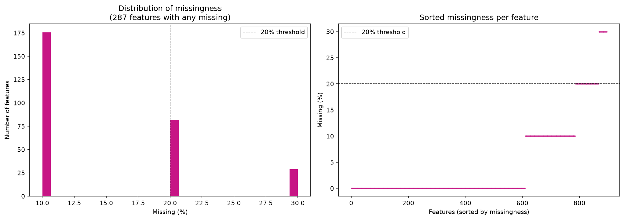
plot_feature_missingness(data_filtered_3)
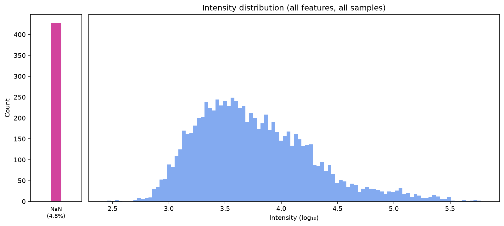
plot_intensity_distribution(data_filtered_3)

Total count of missing cells: 427
Overall percentage of missingness: 4.760312151616499

Impute with half minimum

In this imputation method, we are calculating the minimum of each feature, taking the half of that and using that value to fill in missing values for that feature. This method is implemented in the acore function imputation_half_minimum().

Note: Another commonly used method in metabolomics data imputation is imputing with zeros. This method can also be applied through acore, with the function imputation_zeros().

data_imputed = imputation_half_minimum(data=data_filtered_3)

data_imputed

id	15167360593113340842	6744901733644451055	11872048905895506999	17709464339328039509	13922238524316478464	7261731678087078534	5009880893163685891	14568390051812142800	12965064019618390832	12018024353057911182	...	10081236272997946842	11566491653082879729	1138090438525564760	16421084926908170456	15756805090958850402	6914550508003274460	8218613456253687867	1747965644941981794	8361543175644692425	9120899724421101875
MS_D_POS.mzML	143,542.600	5,886.109	11,476.870	20,796.740	12,335.740	1,841.792	13,084.690	65,376.190	46,063.120	6,191.987	...	3,473.264	274.633	2,858.896	2,421.536	1,222.554	952.219	5,434.947	15,157.630	2,055.739	3,006.401
MS_C_POS.mzML	173,214.200	4,802.169	10,514.190	18,960.890	16,236.390	2,675.053	13,589.740	71,279.240	18,524.640	5,931.635	...	9,403.579	704.575	1,666.042	858.752	1,444.158	1,444.071	5,278.917	14,413.630	1,598.920	1,444.313
MS_E_POS.mzML	89,948.010	5,141.211	10,575.090	21,024.620	17,866.430	2,610.558	12,433.400	52,452.010	59,626.340	5,618.113	...	13,407.410	1,113.405	5,174.449	2,836.493	2,593.458	1,847.802	3,992.441	15,820.330	1,789.678	1,991.497
MS_B_POS.mzML	93,468.920	2,480.739	8,486.273	21,715.490	11,622.170	4,003.669	12,023.290	61,131.850	69,804.600	5,421.544	...	10,555.010	888.467	3,474.066	3,253.217	2,190.118	1,100.630	4,106.935	15,740.730	4,263.249	1,911.875
MS_A_POS.mzML	157,576.200	6,731.292	9,867.111	19,383.730	19,050.570	2,090.373	12,986.100	65,314.800	53,463.480	5,762.296	...	9,976.974	615.012	3,445.868	2,292.947	611.277	476.110	832.952	7,206.815	799.460	722.156
MS_QC_POOL_1_POS.mzML	198,321.300	4,336.047	9,133.133	23,995.310	9,895.060	2,919.634	10,952.520	54,107.960	31,009.850	5,038.122	...	3,473.264	745.005	833.021	2,352.086	1,371.443	476.110	1,773.438	15,014.210	799.460	2,316.048
MS_QC_POOL_4_POS.mzML	207,862.400	4,037.693	9,277.422	23,487.570	11,016.590	3,455.879	11,468.140	58,678.800	36,071.060	5,318.160	...	6,989.383	724.883	4,274.623	858.752	1,310.173	1,025.298	832.952	14,801.370	2,531.686	722.156
MS_QC_POOL_3_POS.mzML	206,423.100	4,297.844	9,498.344	24,143.250	10,479.450	3,532.990	11,710.650	56,706.770	32,887.300	5,395.765	...	6,946.528	274.633	833.021	2,311.549	611.277	476.110	832.952	7,206.815	2,659.393	2,306.081
MS_F_POS.mzML	169,903.500	5,676.127	10,521.120	19,712.100	23,974.610	1,996.034	10,025.950	66,881.700	25,845.320	4,456.026	...	9,844.492	549.266	833.021	1,717.504	1,296.626	1,237.158	5,141.985	15,161.050	1,860.046	1,595.857
MS_QC_POOL_2_POS.mzML	204,664.500	4,517.161	9,515.199	23,829.240	12,349.160	3,553.620	11,306.920	58,920.040	32,103.840	5,273.946	...	3,473.264	274.633	4,513.373	858.752	611.277	1,068.735	1,665.903	7,206.815	799.460	722.156

10 rows × 897 columns

print(f"Total count of missing cells: {data_imputed.isnull().sum().sum()}")
print(
    f"Overall percentage of missingness: {data_imputed.isnull().mean().mean() * 100}\n"
)

print("SUMMARY of imputation changes:")
missingness_summary(data, data_imputed)
plot_intensity_distribution(data_imputed)

Total count of missing cells: 0
Overall percentage of missingness: 0.0

SUMMARY of imputation changes:
Total values      : 130,940
Missing before    : 88,911  (67.9%)
Missing after     : 0  (0.0%)
Features affected : 12010 / 13094
Samples affected  : 10 / 10

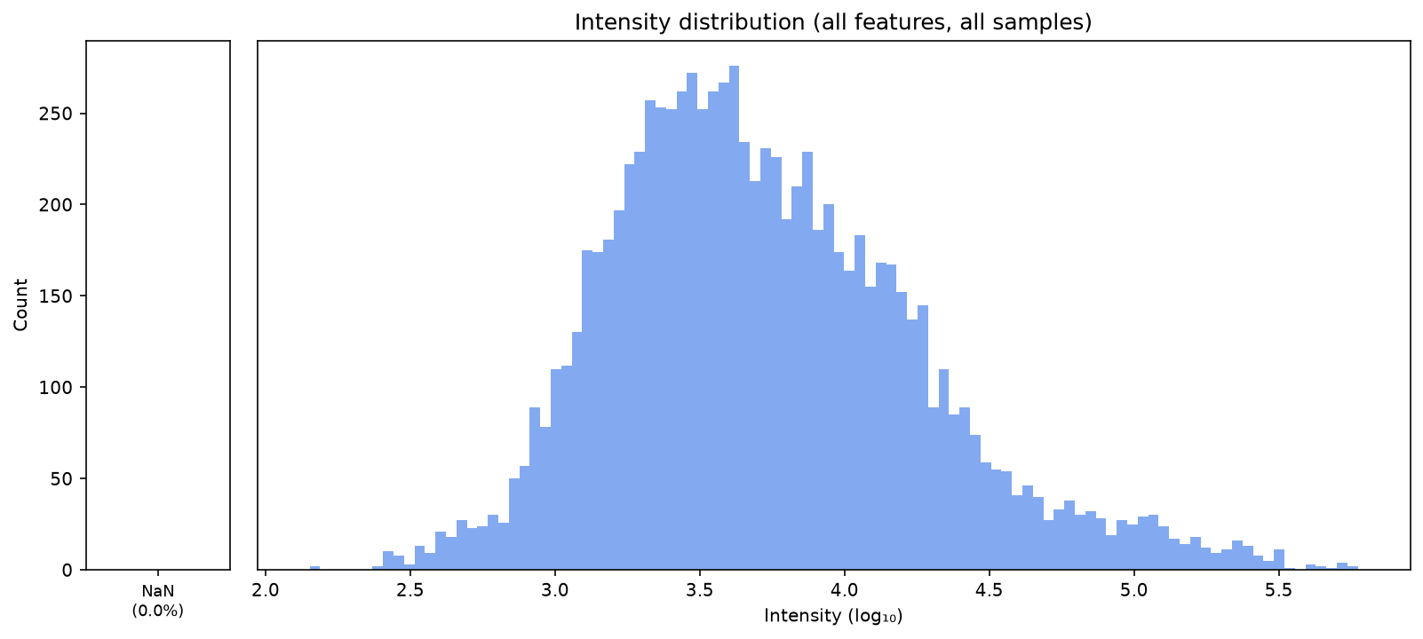
Now we have filled in all missing values. We can now plot the data in a PCA plot to see whether the samples can be separated well with principal components. We can use the functions we defined earlier at the beginning of the notebook for that.

We can plot the PCA first with all samples and QCs, and then with just the samples, to see how the groups separate.

pca_model, scores, var_explained = plot_pca(
    data_imputed, groups_all, label_points=True, title="PCA on imputed data"
)
pca_model, scores, var_explained = plot_pca(
    data_imputed, groups_samples, label_points=True, title="PCA on imputed data"
)

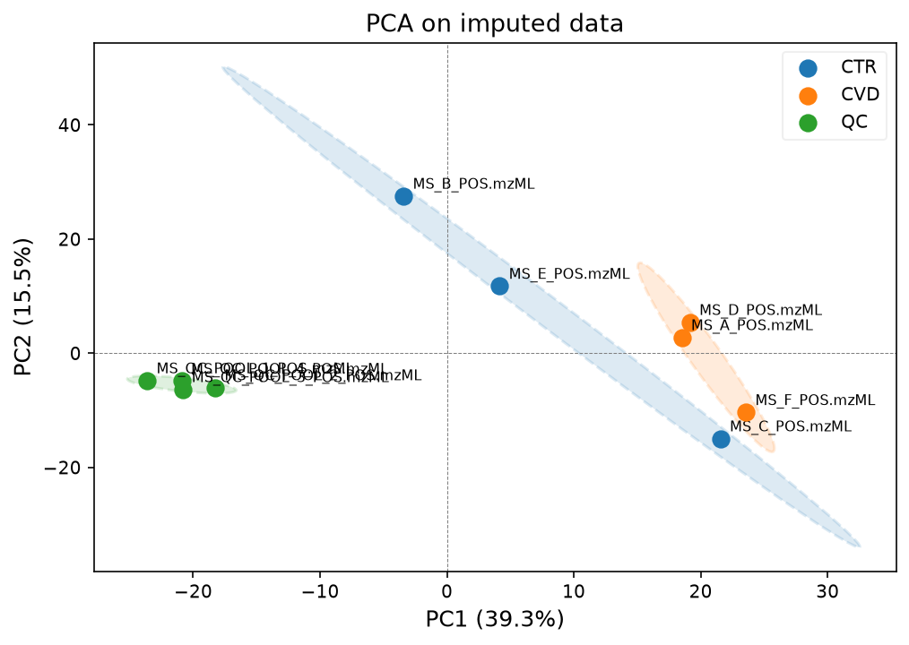
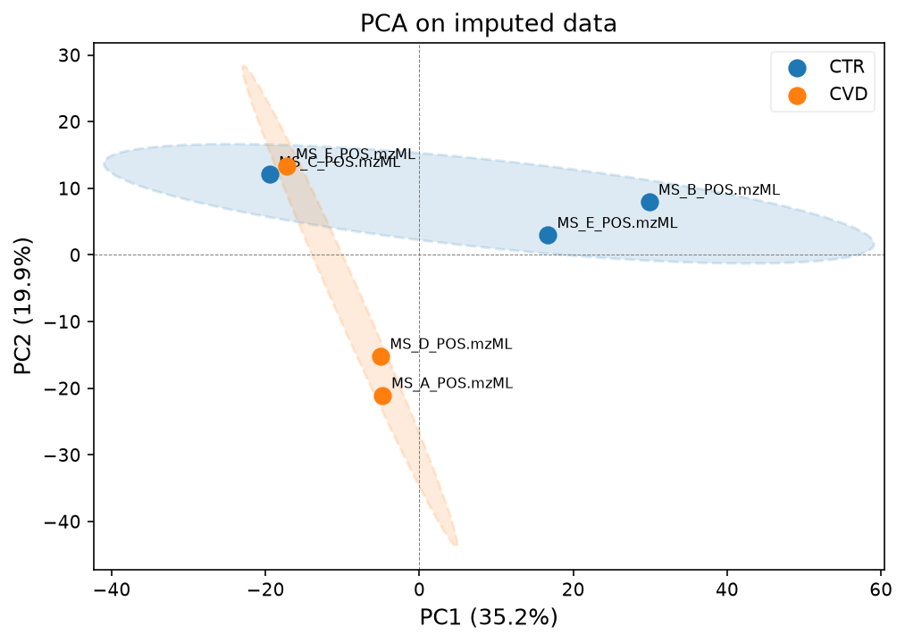
The first plot shows that the QC samples separate quite well from the biological samples.

The second plot shows that the two groups are also separated quite well, although one of the control samples, sample C, clusters slightly away from the rest.

Drift correction

Now that we have a data frame that has been filtered and is fully filled in, we will look at the within-batch effects. In metabolomics, instrumental drift is common, so the signal degrades over time.

This is what we have the QC samples for, which is why they are so important to have included in the study.

We will test two different methods for correcting the instrumental drift in this notebook, inspect the results, and then choose one to continue with.

from acore import drift_correction as dc

Loess smoothing drift correction

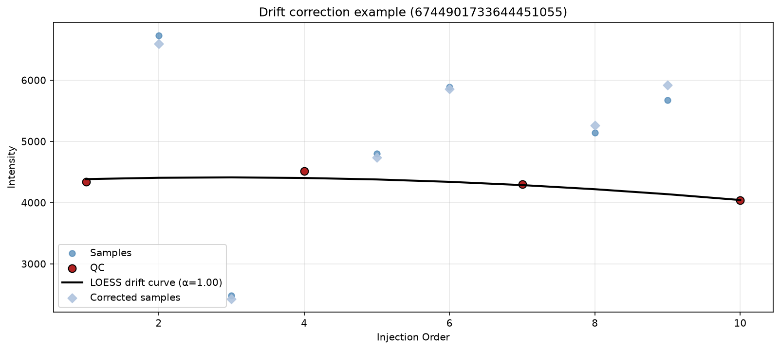
Pooled QC samples are injected at regular intervals over time throughout the experiment. The QC intensities for each features should theoretically be consistent in each measurement. Therefore, any variation in these samples reflect artificial variation, so instrumental drift, instead of biological variation.

LOESS (LOcally Estimated Scatterplot Smoothing) is a non-parametric regression that fits a smooth curve through data without assuming a fixed equation. We use it here to fit a curve over the QC points, and then we rescale the biological sample intensities by the drift estimate. This will be explained better by the visualisations in the real example below.

LOESS smoothing based drift correction is implemented in the loess_drift_correction acore module.

In order to use this method, we need to know the order in which the samples, including QCs, were run. We have this information in our metadata.

sample_order = pd.read_csv(fname_metadata).rename(
    columns={"injection_index": "Sample ID", "derived_spectra_data_file": "File Name"}
)
sample_order

	File Name	phenotype	sample_name	age	Sample ID
0	MS_QC_POOL_1_POS.mzML	QC	POOL1	NaN	1
1	MS_A_POS.mzML	CVD	A	53.000	2
2	MS_B_POS.mzML	CTR	B	30.000	3
3	MS_QC_POOL_2_POS.mzML	QC	POOL2	NaN	4
4	MS_C_POS.mzML	CTR	C	66.000	5
5	MS_D_POS.mzML	CVD	D	36.000	6
6	MS_QC_POOL_3_POS.mzML	QC	POOL3	NaN	7
7	MS_E_POS.mzML	CTR	E	66.000	8
8	MS_F_POS.mzML	CVD	F	44.000	9
9	MS_QC_POOL_4_POS.mzML	QC	POOL4	NaN	10

data_corrected_loess, correction_info = dc.run_loess_drift_correction(
    data=data_imputed, qc_rows=qcs, sample_rows=samples, sample_order=sample_order
)
data_corrected_loess

id	15167360593113340842	6744901733644451055	11872048905895506999	17709464339328039509	13922238524316478464	7261731678087078534	5009880893163685891	14568390051812142800	12965064019618390832	12018024353057911182	...	10081236272997946842	11566491653082879729	1138090438525564760	16421084926908170456	15756805090958850402	6914550508003274460	8218613456253687867	1747965644941981794	8361543175644692425	9120899724421101875
MS_D_POS.mzML	143,573.432	5,855.581	11,405.280	20,793.801	11,825.461	1,844.135	12,982.441	65,407.523	45,379.148	6,168.096	...	3,311.152	365.912	2,681.580	2,471.217	1,527.176	916.919	5,674.860	18,755.105	1,858.585	3,081.469
MS_C_POS.mzML	174,091.915	4,734.838	10,462.922	18,931.842	15,588.876	2,717.426	13,564.355	71,722.861	18,541.397	5,945.064	...	9,868.868	933.982	1,654.844	837.204	1,790.423	1,434.580	4,974.297	17,793.996	1,676.537	1,407.971
MS_E_POS.mzML	89,312.250	5,260.916	10,546.469	21,125.835	17,346.741	2,590.945	12,254.776	52,116.191	56,595.381	5,561.124	...	10,817.891	1,203.488	4,360.125	3,210.646	2,763.118	1,675.787	5,241.677	16,776.352	1,279.548	2,295.194
MS_B_POS.mzML	95,094.860	2,427.454	8,522.518	21,663.213	11,400.772	4,280.714	12,208.936	62,561.603	71,716.179	5,534.163	...	13,814.247	940.708	4,004.152	2,886.022	2,259.722	1,182.188	3,222.823	16,529.271	6,600.248	1,684.365
MS_A_POS.mzML	161,510.647	6,595.786	9,987.575	19,345.144	19,090.120	2,322.102	13,335.245	67,622.219	55,492.351	5,954.525	...	14,814.106	543.880	4,424.151	1,928.941	542.959	539.562	602.743	6,595.115	1,617.820	601.410
MS_QC_POOL_1_POS.mzML	204,976.266	4,269.719	9,339.026	23,969.714	10,213.482	3,403.048	11,393.676	56,809.333	32,456.642	5,281.738	...	5,918.805	540.642	1,240.727	1,864.931	1,029.041	578.280	1,191.074	11,734.965	2,308.962	1,811.879
MS_QC_POOL_4_POS.mzML	205,505.990	4,311.723	9,363.215	23,794.615	11,036.823	3,487.608	11,311.188	58,189.891	32,756.643	5,272.373	...	4,920.639	539.926	3,190.494	1,128.020	1,026.296	866.247	1,419.437	11,724.629	1,522.415	992.605
MS_QC_POOL_3_POS.mzML	205,634.870	4,328.721	9,445.987	24,190.450	10,084.861	3,510.502	11,570.338	56,498.883	31,830.424	5,352.694	...	6,067.819	340.112	740.705	2,476.370	723.792	445.090	971.326	8,453.537	2,119.021	2,495.675
MS_F_POS.mzML	168,278.377	5,922.397	10,544.249	19,879.606	23,593.785	1,991.340	9,876.081	66,353.083	24,015.510	4,409.878	...	7,393.029	497.741	662.707	2,076.658	1,197.659	1,085.413	7,661.980	14,042.548	1,211.548	1,986.662
MS_QC_POOL_2_POS.mzML	206,870.568	4,429.365	9,501.939	23,775.135	11,945.508	3,688.998	11,373.323	59,731.933	32,585.813	5,329.035	...	4,050.263	335.325	4,790.817	799.673	708.475	1,099.972	1,427.385	8,398.979	999.685	669.995

10 rows × 897 columns

Our dataframe has the same structure as before.

We can also look at the object correction_info, if we want to trace the exact correction that was applied to every feature.

correction_info[data_corrected_loess.columns[0]]

{'alpha': np.float64(0.9999999999999999),
 'drift_curve': [207528.80858189552,
  207006.94258480993,
  204507.5144035575,
  200536.6918229344,
  202029.39468897512,
  205499.65973918274,
  198870.40795967163,
  203351.88080133556,
  206331.68105175294,
  207900.64328655135],
 'y_qc': [198321.3, 204664.5, 206423.1, 207862.4],
 'x_qc': [1, 4, 7, 10],
 'rsd_qc': np.float64(1.7828199375522682),
 'median': np.float64(205543.8),
 'y_all': [169903.5,
  89948.01,
  173214.2,
  157576.2,
  93468.92,
  143542.6,
  198321.3,
  204664.5,
  206423.1,
  207862.4],
 'new_values': [168278.37668387496,
  89312.2498549218,
  174091.9153303282,
  161510.64746873346,
  95094.85997457383,
  143573.43220580718,
  204976.26590682287,
  206870.56785178115,
  205634.86986343015,
  205505.99025435423],
 'status': 'corrected'}

To understand better what is happening, we can plot a single feature with all its measurements over time, and the loess curve that is calculated over it. We can try out a few different features to see what would happen, and also try different smoothing parameters to see how the curve changes.

plot_loess_example_curve(
    df=data_imputed,
    feature_idx=1,
    samples=samples,
    qcs=qcs,
    sample_order=sample_order,
)

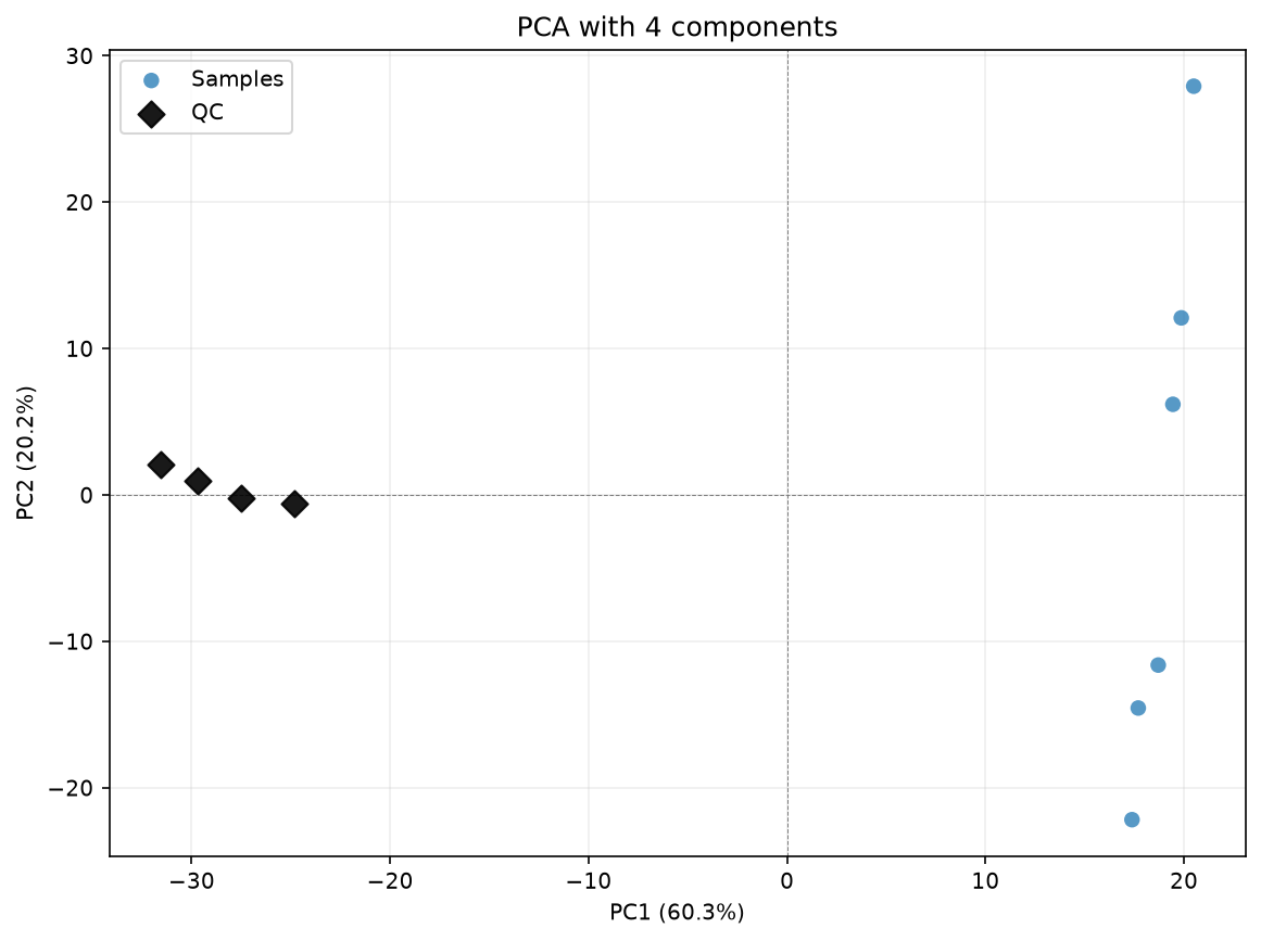
CPCA

Standard PCA finds orthogonal directions (principal components) that capture maximum variance in a single dataset. Common PCA extends this to multiple groups: instead of computing separate components per batch, it tries to find a set of components that are common across groups.

In this case, it finds the principal components that are common across all samples, because the assumption is that those are the ones that are due to artificial variation, whereas the variance in biological samples will not be shared across all.

First, we can plot a PCA for this purpose.

pca_for_cpca_drift(
    data_imputed,
    samples=samples,  # list of col names, OR dict {group_name: [col names]}
    qcs=qcs,
    log_transform=True,
    title="PCA",
)

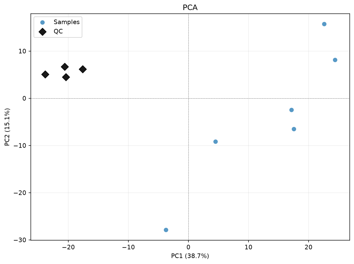
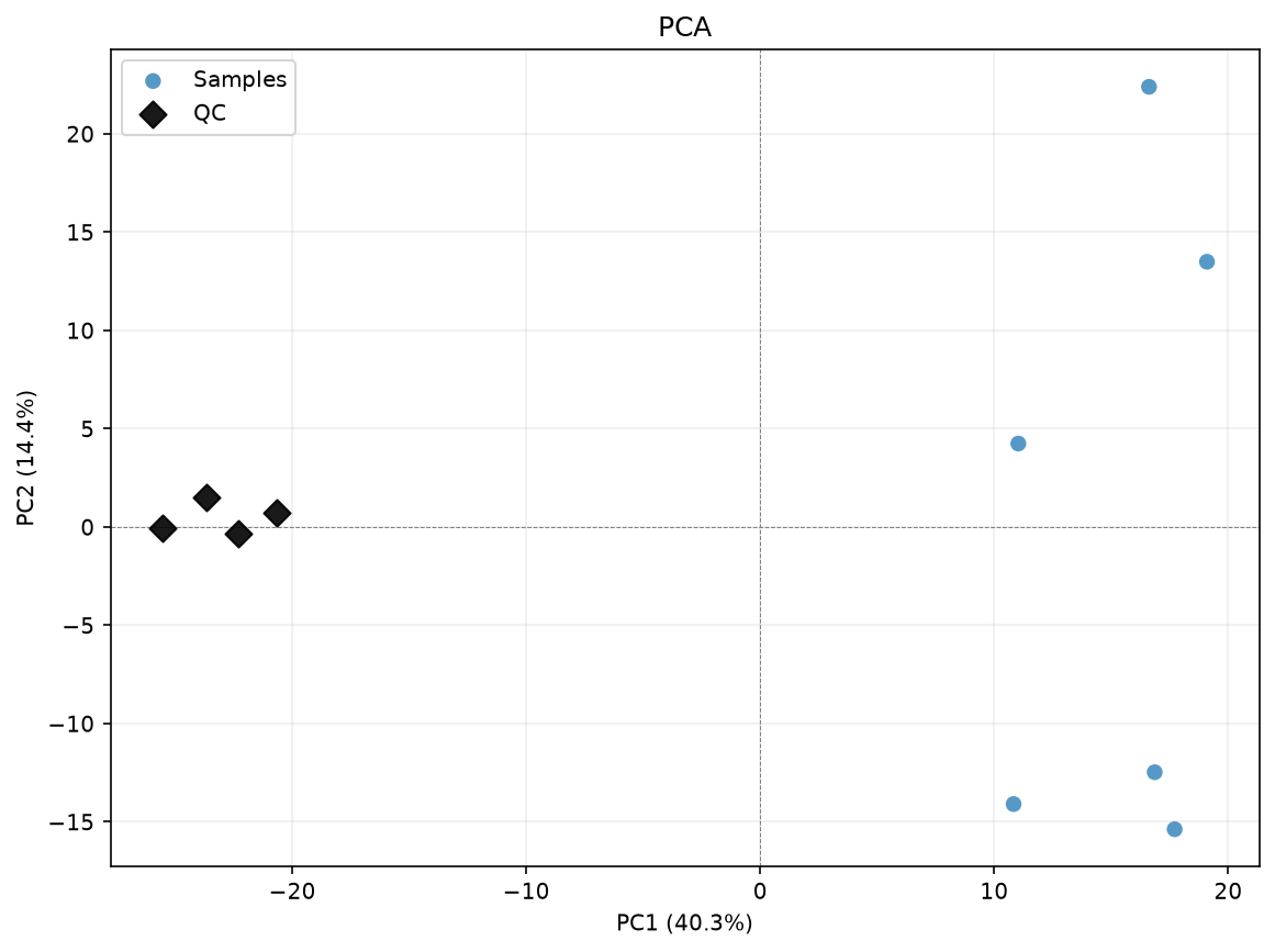
The QC samples are already quite close together, but there is some variation.

We can use the acore function cpca_drift_correction for this.

data_corrected_cpca = dc.run_cpca_drift_correction(
    data_imputed, sample_rows=samples, qc_rows=qcs, n_comps=1
)

pca_for_cpca_drift(
    data_corrected_cpca,
    samples=samples,  # list of col names, OR dict {group_name: [col names]}
    qcs=qcs,
    log_transform=True,
    title="PCA",
)

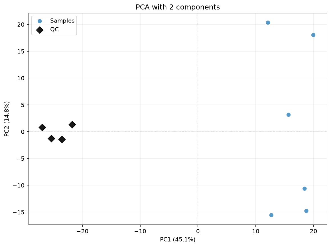
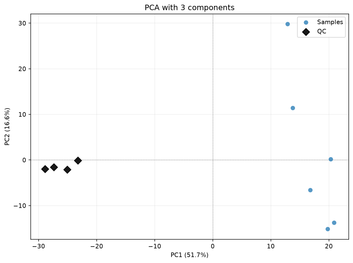
df_corrected_2comps = dc.run_cpca_drift_correction(
    data_imputed, samples, qcs, n_comps=2
)
df_corrected_3comps = dc.run_cpca_drift_correction(
    data_imputed, samples, qcs, n_comps=3
)
df_corrected_4comps = dc.run_cpca_drift_correction(
    data_imputed, samples, qcs, n_comps=4
)

pca_for_cpca_drift(
    df_corrected_2comps,
    samples,
    qcs,
    log_transform=True,
    title="PCA with 2 components",
)

pca_for_cpca_drift(
    df_corrected_3comps,
    samples,
    qcs,
    log_transform=True,
    title="PCA with 3 components",
)

pca_for_cpca_drift(
    df_corrected_4comps,
    samples,
    qcs,
    log_transform=True,
    title="PCA with 4 components",
)

pca_model, scores, var_explained = plot_pca(
    data_corrected_loess,
    groups_all,
    label_points=True,
    title="PCA on LOESS-corrected data",
)
pca_model, scores, var_explained = plot_pca(
    data_corrected_loess,
    groups_samples,
    label_points=True,
    title="PCA on LOESS-corrected data",
)
pca_model, scores, var_explained = plot_pca(
    data_corrected_cpca,
    groups_all,
    label_points=True,
    title="PCA on CPCA-corrected data",
)
pca_model, scores, var_explained = plot_pca(
    data_corrected_cpca,
    groups_samples,
    label_points=True,
    title="PCA on CPCA-corrected data",
)

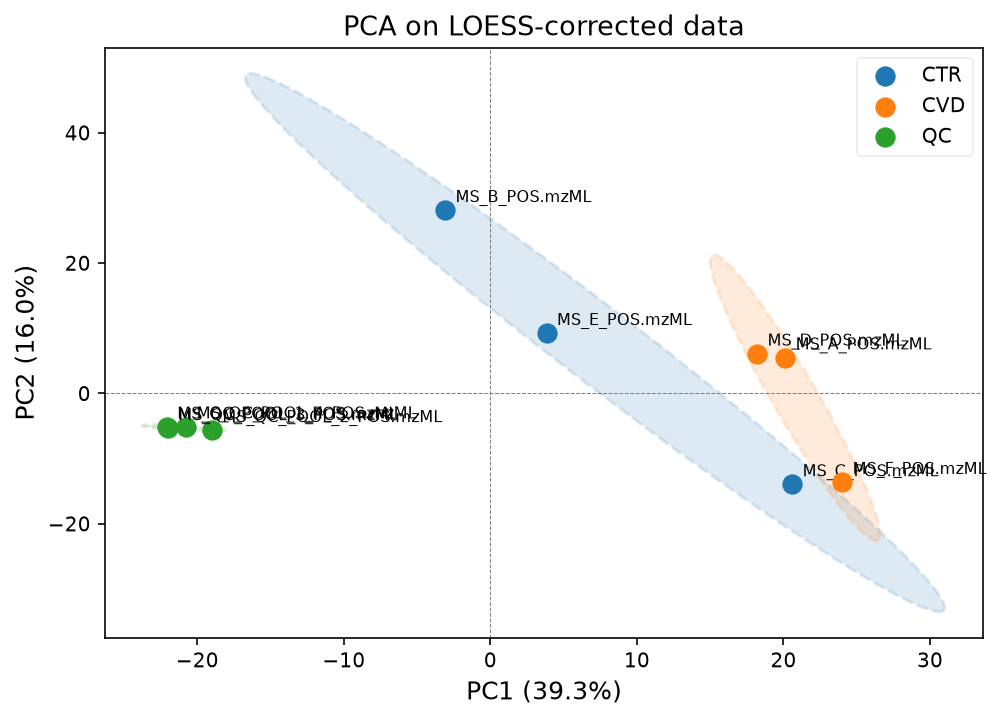
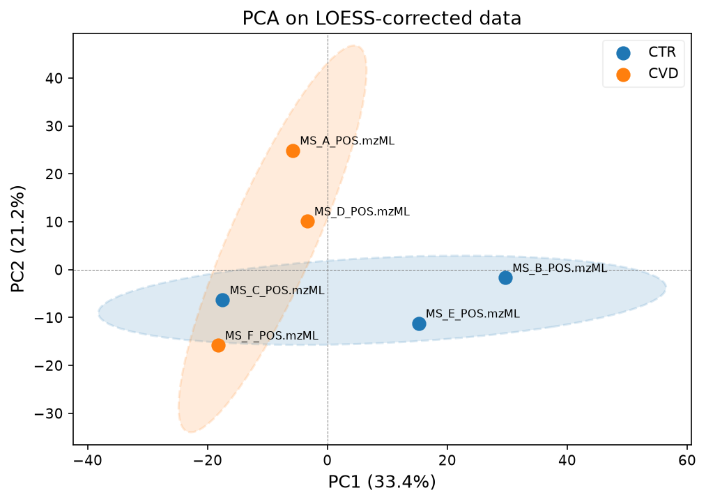
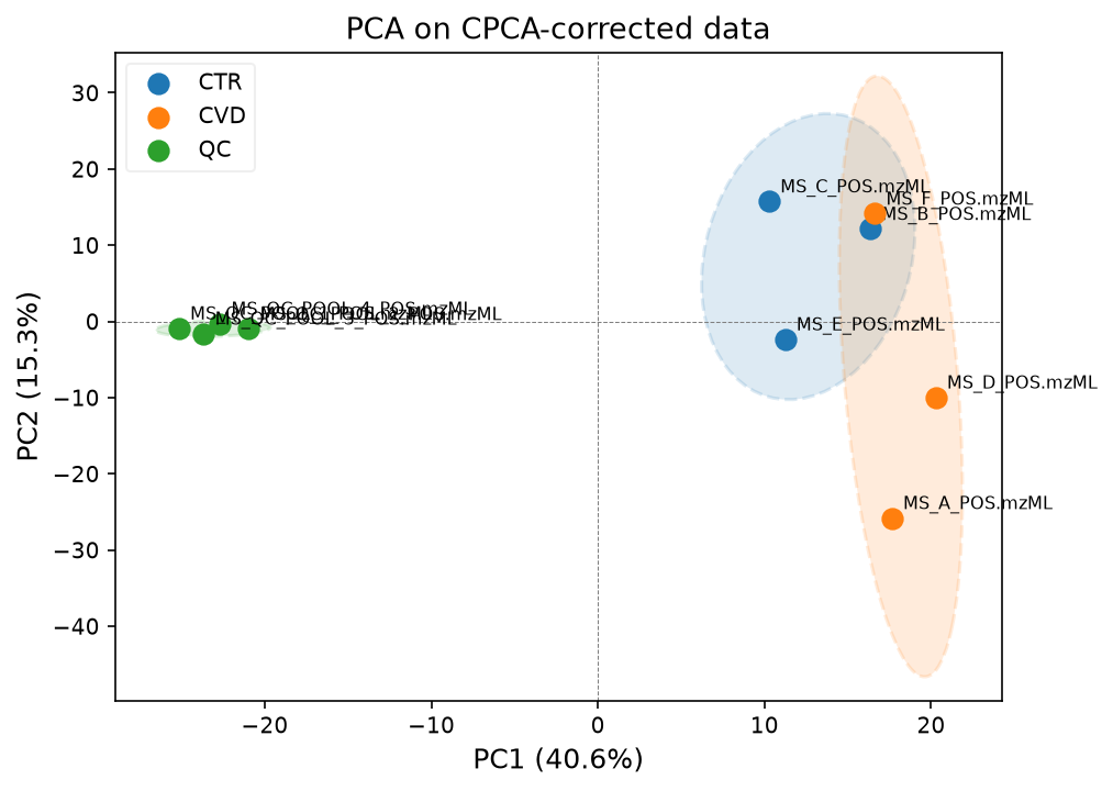
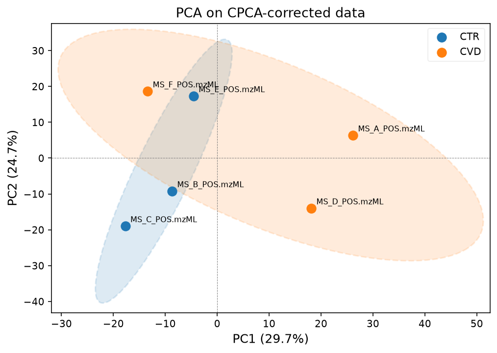
We will continue with the LOESS corrected data.

Normalization

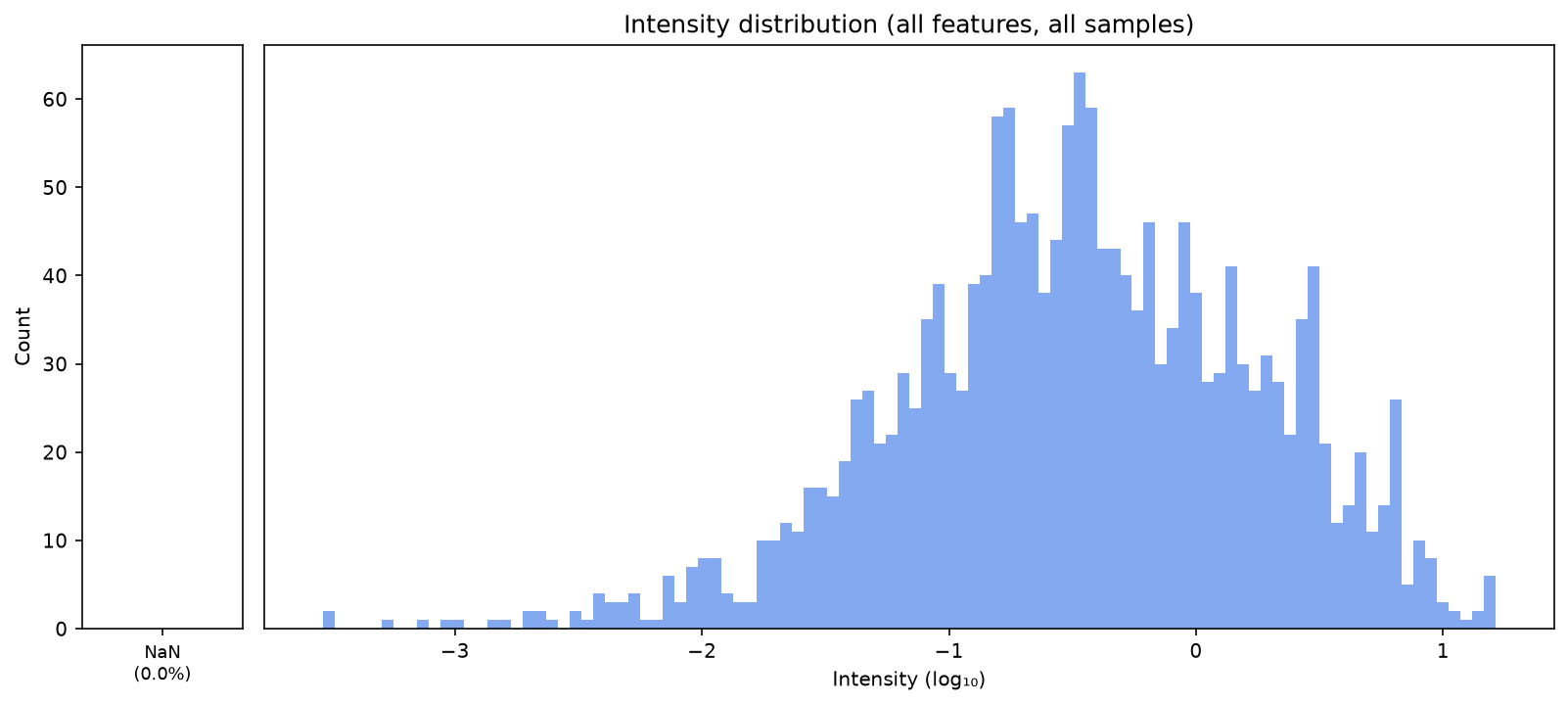
We will also normalise the data with Z-score normalisation. In this case, this will be mainly for visualisation purposes, again to see whether the data is separating well.

We will use an acore function for this again.

from acore import normalization

data_normalized = normalization.normalize_data(data_corrected_loess, "zscore")
data_normalized

id	15167360593113340842	6744901733644451055	11872048905895506999	17709464339328039509	13922238524316478464	7261731678087078534	5009880893163685891	14568390051812142800	12965064019618390832	12018024353057911182	...	10081236272997946842	11566491653082879729	1138090438525564760	16421084926908170456	15756805090958850402	6914550508003274460	8218613456253687867	1747965644941981794	8361543175644692425	9120899724421101875
MS_D_POS.mzML	3.599	-0.255	-0.100	0.163	-0.088	-0.367	-0.056	1.411	0.851	-0.246	...	-0.326	-0.409	-0.344	-0.350	-0.376	-0.393	-0.260	0.106	-0.367	-0.333
MS_C_POS.mzML	4.191	-0.261	-0.111	0.112	0.024	-0.314	-0.029	1.500	0.102	-0.230	...	-0.126	-0.361	-0.342	-0.364	-0.339	-0.348	-0.255	0.082	-0.342	-0.349
MS_E_POS.mzML	2.115	-0.268	-0.119	0.181	0.074	-0.344	-0.070	1.060	1.187	-0.260	...	-0.111	-0.383	-0.294	-0.327	-0.339	-0.370	-0.269	0.058	-0.381	-0.353
MS_B_POS.mzML	2.247	-0.325	-0.156	0.209	-0.076	-0.274	-0.054	1.344	1.598	-0.239	...	-0.009	-0.366	-0.281	-0.312	-0.330	-0.360	-0.303	0.066	-0.209	-0.346
MS_A_POS.mzML	3.913	-0.244	-0.153	0.098	0.091	-0.359	-0.063	1.393	1.068	-0.261	...	-0.024	-0.407	-0.303	-0.370	-0.407	-0.407	-0.405	-0.244	-0.378	-0.405
MS_QC_POOL_1_POS.mzML	5.824	-0.260	-0.106	0.337	-0.080	-0.286	-0.044	1.333	0.594	-0.229	...	-0.210	-0.373	-0.352	-0.333	-0.358	-0.372	-0.353	-0.034	-0.320	-0.335
MS_QC_POOL_4_POS.mzML	5.779	-0.261	-0.109	0.324	-0.059	-0.285	-0.051	1.357	0.593	-0.232	...	-0.242	-0.374	-0.294	-0.356	-0.359	-0.364	-0.348	-0.038	-0.344	-0.360
MS_QC_POOL_3_POS.mzML	5.791	-0.255	-0.102	0.341	-0.082	-0.280	-0.038	1.312	0.571	-0.225	...	-0.203	-0.375	-0.363	-0.311	-0.364	-0.372	-0.356	-0.131	-0.322	-0.310
MS_F_POS.mzML	4.348	-0.243	-0.112	0.152	0.257	-0.354	-0.131	1.466	0.269	-0.286	...	-0.201	-0.396	-0.392	-0.352	-0.376	-0.380	-0.194	-0.013	-0.376	-0.354
MS_QC_POOL_2_POS.mzML	5.698	-0.256	-0.107	0.313	-0.035	-0.278	-0.052	1.370	0.572	-0.230	...	-0.268	-0.377	-0.246	-0.363	-0.366	-0.354	-0.345	-0.140	-0.357	-0.367

10 rows × 897 columns

plot_intensity_distribution(data_normalized)

pca_model, scores, var_explained = plot_pca(
    data_normalized, groups_all, label_points=True, title="PCA on normalized data"
)
pca_model, scores, var_explained = plot_pca(
    data_normalized, groups_samples, label_points=True, title="PCA on normalized data"
)

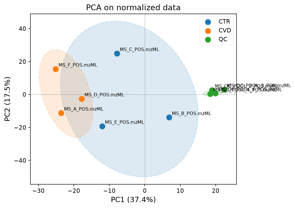
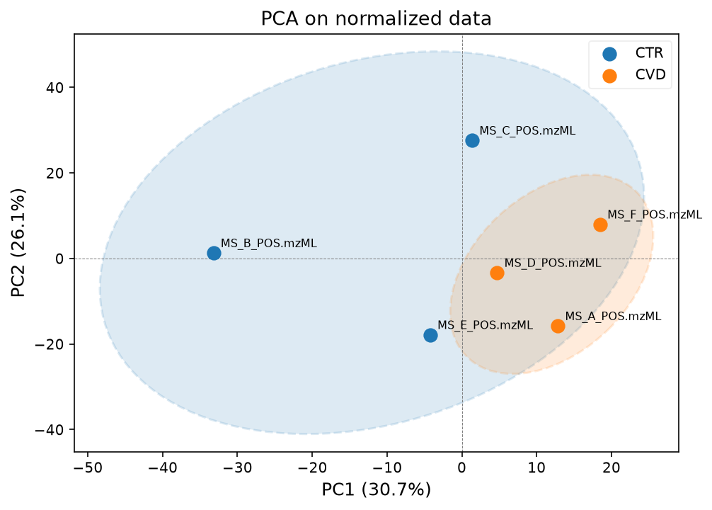
We can see that sample C is still distorting the separation. To know what went wrong with this control, we would need to know more about the sample preparation and background about the patients.

Statistical analysis

ANCOVA

We will now do a statistical analysis. We want to find out which ones of our metabolites are significantly more abundant in the cardiovascular disease group vs the control, or the other way around.

For this, we will do an ANCOVA (analysis of covariance), which compares group means on an outcome while statistically controlling for one or more continuous variables (covariates) that also influence the outcome. In this case, the covariate is age, because we have this in our metadata and know that it could potentially affect the sample outcomes.

We are using another acore function for this.

import acore.differential_regulation as ad

We need to do some preparation before we can run the function.

# Create the variable with the data
data_ancova = np.log2(data_imputed)

# Prepare the data to fit the function input
subject_col = data_ancova.index.name or "index"
data_ancova.rename_axis(subject_col, axis=0, inplace=True)

# Add group information to the data frame as a column
group_map = {
    sample: label for label, samples in groups_all.items() for sample in samples
}
data_ancova.insert(0, "group", data_ancova.index.map(group_map))

# Remove the QC samples
data_ancova = data_ancova[data_ancova["group"] != "QC"]

# Add the column of age information
metadata = sample_order.copy().set_index("File Name")
data_ancova.insert(1, "age", metadata.loc[data_ancova.index, "age"])

data_ancova

id	group	age	15167360593113340842	6744901733644451055	11872048905895506999	17709464339328039509	13922238524316478464	7261731678087078534	5009880893163685891	14568390051812142800	...	10081236272997946842	11566491653082879729	1138090438525564760	16421084926908170456	15756805090958850402	6914550508003274460	8218613456253687867	1747965644941981794	8361543175644692425	9120899724421101875
index
MS_D_POS.mzML	CVD	36.000	17.131	12.523	13.486	14.344	13.591	10.847	13.676	15.996	...	11.762	8.101	11.481	11.242	10.256	9.895	12.408	13.888	11.005	11.554
MS_C_POS.mzML	CTR	66.000	17.402	12.229	13.360	14.211	13.987	11.385	13.730	16.121	...	13.199	9.461	10.702	9.746	10.496	10.496	12.366	13.815	10.643	10.496
MS_E_POS.mzML	CTR	66.000	16.457	12.328	13.368	14.360	14.125	11.350	13.602	15.679	...	13.711	10.121	12.337	11.470	11.341	10.852	11.963	13.949	10.805	10.960
MS_B_POS.mzML	CTR	30.000	16.512	11.277	13.051	14.406	13.505	11.967	13.554	15.900	...	13.366	9.795	11.762	11.668	11.097	10.104	12.004	13.942	12.058	10.901
MS_A_POS.mzML	CVD	53.000	17.266	12.717	13.268	14.243	14.218	11.030	13.665	15.995	...	13.284	9.264	11.751	11.163	9.256	8.895	9.702	12.815	9.643	9.496
MS_F_POS.mzML	CVD	44.000	17.374	12.471	13.361	14.267	14.549	10.963	13.291	16.029	...	13.265	9.101	9.702	10.746	10.341	10.273	12.328	13.888	10.861	10.640

6 rows × 899 columns

Now we can run ANCOVA.

ancova = (
    ad.run_ancova(
        data_ancova.astype({"group": str}),  # ! target needs to be of type str
        # subject=subject_col, # not used
        drop_cols=[],
        group="group",  # needs to be a string
        covariates=["age"],
    )
    .set_index("identifier")
    .sort_values(by="padj")
)  # need to be floats?
ancova

	group1	group2	mean(group1)	std(group1)	mean(group2)	std(group2)	posthoc T-Statistics	posthoc pvalue	coef	std err	...	log2FC	FC	F-statistics	pvalue	padj	correction	rejected	-log10 pvalue	Method	posthoc padj
identifier
8688552057745683191	CTR	CVD	12.353	0.637	13.042	0.299	15.878	0.001	0.874	0.055	...	-0.689	0.620	252.110	0.001	0.194	FDR correction BH	False	3.265	One-way ancova	0.194
4803564648587047687	CTR	CVD	12.092	0.044	11.818	0.021	-13.572	0.001	-0.284	0.021	...	0.274	1.209	184.207	0.001	0.194	FDR correction BH	False	3.063	One-way ancova	0.194
122927701965791210	CTR	CVD	13.368	0.809	14.097	0.306	14.470	0.001	0.957	0.066	...	-0.729	0.603	209.372	0.001	0.194	FDR correction BH	False	3.145	One-way ancova	0.194
14183644523572007298	CTR	CVD	11.362	0.828	12.072	0.356	21.223	0.000	0.948	0.045	...	-0.710	0.611	450.404	0.000	0.194	FDR correction BH	False	3.640	One-way ancova	0.194
16452322344680482043	CTR	CVD	14.418	0.588	15.296	0.362	7.963	0.004	1.054	0.132	...	-0.879	0.544	63.409	0.004	0.318	FDR correction BH	False	2.384	One-way ancova	0.318
...	...	...	...	...	...	...	...	...	...	...	...	...	...	...	...	...	...	...	...	...	...
15322232151823440986	CTR	CVD	12.649	0.145	12.693	0.164	0.027	0.980	0.003	0.106	...	-0.044	0.970	0.001	0.980	0.992	FDR correction BH	False	0.009	One-way ancova	0.992
13146520139614759536	CTR	CVD	11.517	0.213	11.555	0.121	0.010	0.993	0.001	0.138	...	-0.038	0.974	0.000	0.993	0.994	FDR correction BH	False	0.003	One-way ancova	0.994
3927519029408433709	CTR	CVD	13.941	0.112	13.919	0.142	-0.009	0.993	-0.001	0.111	...	0.022	1.015	0.000	0.993	0.994	FDR correction BH	False	0.003	One-way ancova	0.994
18162318233842994935	CTR	CVD	13.669	0.374	13.720	0.325	-0.012	0.991	-0.004	0.308	...	-0.051	0.965	0.000	0.991	0.994	FDR correction BH	False	0.004	One-way ancova	0.994
491936035475549414	CTR	CVD	11.796	2.677	12.144	2.116	0.005	0.996	0.010	2.165	...	-0.348	0.786	0.000	0.996	0.996	FDR correction BH	False	0.002	One-way ancova	0.996

897 rows × 22 columns

We have filtered the table by the adjusted pvalue. We can look at the top values to see how good our best hits are. We are sorting the data by the adjusted pvalue to see what our best hits are, and how good they actually are. In this case, our best hits have adjusted pvalues of 0.321 and higher, which is quite high, and not significant.

We can inspect the results in a few different ways. First of all, we can look at the group averages, which are shown in the first six columns.

ancova.iloc[:, :6]

	group1	group2	mean(group1)	std(group1)	mean(group2)	std(group2)
identifier
8688552057745683191	CTR	CVD	12.353	0.637	13.042	0.299
4803564648587047687	CTR	CVD	12.092	0.044	11.818	0.021
122927701965791210	CTR	CVD	13.368	0.809	14.097	0.306
14183644523572007298	CTR	CVD	11.362	0.828	12.072	0.356
16452322344680482043	CTR	CVD	14.418	0.588	15.296	0.362
...	...	...	...	...	...	...
15322232151823440986	CTR	CVD	12.649	0.145	12.693	0.164
13146520139614759536	CTR	CVD	11.517	0.213	11.555	0.121
3927519029408433709	CTR	CVD	13.941	0.112	13.919	0.142
18162318233842994935	CTR	CVD	13.669	0.374	13.720	0.325
491936035475549414	CTR	CVD	11.796	2.677	12.144	2.116

897 rows × 6 columns

If we filter to the words below, we can inspect the test results (based on a linear model) for each feature (on each row). The posthoc values are not interesting in this case as we are only comparing between two groups (ctr and cvd). We are mainly interested in the adjusted pvalue (pajd), and in whether the null hypothesis was rejected or not. If rejected=True, it means our feature was significant according to the thresholds we have set.

regex_filter = "pval|padj|reject|post"
ancova.filter(regex=regex_filter)

	posthoc T-Statistics	posthoc pvalue	pvalue	padj	rejected	-log10 pvalue	posthoc padj
identifier
8688552057745683191	15.878	0.001	0.001	0.194	False	3.265	0.194
4803564648587047687	-13.572	0.001	0.001	0.194	False	3.063	0.194
122927701965791210	14.470	0.001	0.001	0.194	False	3.145	0.194
14183644523572007298	21.223	0.000	0.000	0.194	False	3.640	0.194
16452322344680482043	7.963	0.004	0.004	0.318	False	2.384	0.318
...	...	...	...	...	...	...	...
15322232151823440986	0.027	0.980	0.980	0.992	False	0.009	0.992
13146520139614759536	0.010	0.993	0.993	0.994	False	0.003	0.994
3927519029408433709	-0.009	0.993	0.993	0.994	False	0.003	0.994
18162318233842994935	-0.012	0.991	0.991	0.994	False	0.004	0.994
491936035475549414	0.005	0.996	0.996	0.996	False	0.002	0.996

897 rows × 7 columns

As we could already see by the high adjusted pvalues in the data frame, none of the values are significant, which is why rejected=False for all of them.

You can also look at the rest of the results.

ancova.iloc[:, 6:].filter(regex=f"^(?!.*({regex_filter})).*$")

	coef	std err	Conf. Int. Low	Conf. Int. Upp.	log2FC	FC	F-statistics	correction	Method
identifier
8688552057745683191	0.874	0.055	0.699	1.049	-0.689	0.620	252.110	FDR correction BH	One-way ancova
4803564648587047687	-0.284	0.021	-0.351	-0.218	0.274	1.209	184.207	FDR correction BH	One-way ancova
122927701965791210	0.957	0.066	0.746	1.167	-0.729	0.603	209.372	FDR correction BH	One-way ancova
14183644523572007298	0.948	0.045	0.806	1.090	-0.710	0.611	450.404	FDR correction BH	One-way ancova
16452322344680482043	1.054	0.132	0.633	1.476	-0.879	0.544	63.409	FDR correction BH	One-way ancova
...	...	...	...	...	...	...	...	...	...
15322232151823440986	0.003	0.106	-0.334	0.340	-0.044	0.970	0.001	FDR correction BH	One-way ancova
13146520139614759536	0.001	0.138	-0.438	0.441	-0.038	0.974	0.000	FDR correction BH	One-way ancova
3927519029408433709	-0.001	0.111	-0.355	0.353	0.022	1.015	0.000	FDR correction BH	One-way ancova
18162318233842994935	-0.004	0.308	-0.984	0.977	-0.051	0.965	0.000	FDR correction BH	One-way ancova
491936035475549414	0.010	2.165	-6.881	6.901	-0.348	0.786	0.000	FDR correction BH	One-way ancova

897 rows × 9 columns

Now we can plot a volcano plot, which is a scatter plot that combines statistical significance and effect size (magnitude of change) in a single view.

scatter_plot_adv = vuecore.plots.basic.scatter.create_scatter_plot(
    data=ancova.reset_index(),
    x="log2FC",
    y="-log10 pvalue",
    color="rejected",
    title="Volcano Plot showing CTR vs CVD samples",
    subtitle="Visualizing ANCOVA results",
    labels={
        "log2FC": "Log2 Fold Change",
        "-log10 pvalue": "-log10(p-value)",
        "pvalue": "Raw P value",
        "rejected": "FDR corrected Significant",
        "identifier": "Feature Identifier",
    },
    hover_data=["identifier"],
    # currently does not work:
    # color_discrete_map={False: "#2166AC", True: "#B2182B"},  # Blue  # Red
    color_discrete_sequence=["red", "blue"],
    opacity=1,
    marker_line_width=1,
    marker_line_color="darkgray",
    width=800,
    height=600,
)
scatter_plot_adv

If we had significant values, they would show up in blue in this plot.

fig, axes = plt.subplots(1, 2, figsize=(12, 5))

# Raw p-values
axes[0].hist(
    ancova["pvalue"].dropna(),
    bins=50,
    color="steelblue",
    edgecolor="white",
    linewidth=0.5,
)
axes[0].set_title("Distribution of Raw P-values", fontsize=14, fontweight="bold")
axes[0].set_xlabel("Raw p-value")
axes[0].set_ylabel("Count")
axes[0].axvline(x=0.05, color="red", linestyle="--", linewidth=1.5, label="α = 0.05")
axes[0].legend()

# Adjusted p-values
axes[1].hist(
    ancova["padj"].dropna(),
    bins=50,
    color="darkorange",
    edgecolor="white",
    linewidth=0.5,
)
axes[1].set_title(
    "Distribution of Adjusted P-values (FDR correction BH)",
    fontsize=14,
    fontweight="bold",
)
axes[1].set_xlabel("Adjusted p-value")
axes[1].set_ylabel("Count")
axes[1].axvline(x=0.05, color="red", linestyle="--", linewidth=1.5, label="α = 0.05")
axes[1].legend()


plt.suptitle("P-value Distributions", fontsize=16, fontweight="bold", y=1.02)
plt.tight_layout()
plt.show()

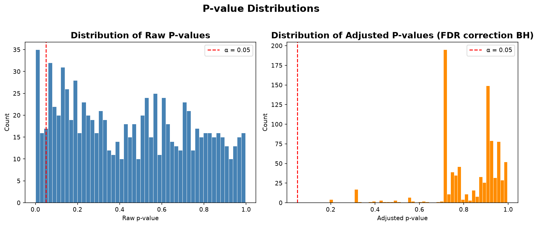
In the above plot, we are looking at our pvalues and adjusted pvalues in more detail.

We can also see how many features survived each threshold in the calculations below.

print("Raw p < 0.05:", (ancova["pvalue"] < 0.05).sum())
print("Raw p < 0.01:", (ancova["pvalue"] < 0.01).sum())
print("padj < 0.05: ", (ancova["padj"] < 0.05).sum())
print("padj < 0.1:  ", (ancova["padj"] < 0.1).sum())

Raw p < 0.05: 58
Raw p < 0.01: 23
padj < 0.05:  0
padj < 0.1:   0

Identify hits

Finally, we can identify our best hits to then be analysed further. Once we have found our top hits, we can match the (for now unknown) features with library spectra and identify which metabolites they are. Then, we can carry out further analyses such as enrichment analysis.

We can choose some thresholds for this, often we would choose an adjusted pvalue of 0.05 or lower, and an absolute log2 fold change of 1 or higher.

# Primary hit list for follow-up
hits = ancova[(ancova["padj"] < 0.05) & (ancova["log2FC"].abs() > 1)]
print(f"Candidate metabolites: {len(hits)}")
print(f"Upregulated in CVD: {(hits['log2FC'] > 0).sum()}")
print(f"Downregulated in CVD: {(hits['log2FC'] < 0).sum()}")

Candidate metabolites: 0
Upregulated in CVD: 0
Downregulated in CVD: 0

We can save and export our hits to a csv file. Usually we would save the top hits and explore them further, but in this case, we will save the whole ancova, and just look further into the top metabolites here, although they are not significant.

ancova.to_csv("results_prepared/ancova_results.csv")

Done!