5.5 Part 2 — Gene Set Enrichment Analysis (GSEA) | Introduction to Transcriptomics

5.5 Part 2 — Gene Set Enrichment Analysis (GSEA)

What is GSEA?

GSEA asks: “Are genes in a pathway coordinately shifting up or down across my full ranked list?”

Unlike ORA, GSEA:

Uses all tested genes — capturing coordinated but subtle pathway-level changes
Ranks genes by a metric encoding both significance and direction
Returns a Normalised Enrichment Score (NES): positive NES = pathway upregulated in treatment; negative NES = pathway downregulated

Why signed log p-value for ranking?

rank = sign(LFC) x -log10(pvalue)

Genes at the top are significantly upregulated; genes at the bottom are significantly downregulated. This is more robust than ranking on LFC alone, which can place noisy high-fold-change genes from lowly expressed genes at the extremes.

📘 Note: Genes with pvalue = 0 (below machine precision in DESeq2) are excluded because -log10(0) = Inf is not a valid ranking score. These are the most extremely significant genes and their exclusion has minimal impact on pathway-level results.

5.5.1 Prepare the Ranked Gene List

ranked_df <- res_df_sym %>%
  filter(!is.na(pvalue), !is.na(log2FoldChange)) %>%
  filter(pvalue > 0) %>%                    # exclude p=0 -> log10(0) = Inf
  mutate(rank_metric = sign(log2FoldChange) * -log10(pvalue)) %>%
  arrange(desc(rank_metric)) %>%
  distinct(gene, .keep_all = TRUE)

rank_vector        <- ranked_df$rank_metric
names(rank_vector) <- ranked_df$gene

cat("Genes in ranked list :", length(rank_vector), "\n")

## Genes in ranked list : 3697

cat("Infinite values      :", sum(!is.finite(rank_vector)), "\n")

## Infinite values      : 0

cat("Top 5 (upregulated)  :", paste(head(names(rank_vector), 5), collapse = ", "), "\n")

## Top 5 (upregulated)  : b3508, b3510, gadC, b3509, gadB

cat("Bottom 5 (downreg.)  :", paste(tail(names(rank_vector), 5), collapse = ", "), "\n")

## Bottom 5 (downreg.)  : mglB, garL, b3127, b0553, garR

5.5.2 Convert GMT to fgsea Format

fgsea requires a named list of gene vectors — one entry per pathway.

pathways_list <- setNames(
  kegg_gmt$list_of_values,
  kegg_gmt$ontology_name
)

cat("Pathways in list:", length(pathways_list), "\n")

## Pathways in list: 121

cat("Example entry   :", pathways_list[[1]][1:5], "\n")

## Example entry   : aceE aceF lpd yahK frmA

5.5.3 Run GSEA

set.seed(42)

gsea_results <- fgsea(
  pathways    = pathways_list,
  stats       = rank_vector,
  minSize     = 10,
  maxSize     = 500,
  nPermSimple = 10000
)

cat("Pathways tested          :", nrow(gsea_results), "\n")

## Pathways tested          : 77

cat("Significant (padj < 0.05):", sum(gsea_results$padj < 0.05, na.rm = TRUE), "\n")

## Significant (padj < 0.05): 2

cat("Nominal (pval < 0.05)    :", sum(gsea_results$pval < 0.05, na.rm = TRUE), "\n")

## Nominal (pval < 0.05)    : 18

5.5.4 Filter and Inspect Significant Pathways

gsea_sig <- gsea_results %>%
  as.data.frame() %>%
  filter(padj < 0.05) %>%
  arrange(padj)

cat("Significant GSEA pathways:", nrow(gsea_sig), "\n")

## Significant GSEA pathways: 2

cat("  Activated (NES > 0)    :", sum(gsea_sig$NES > 0), "\n")

##   Activated (NES > 0)    : 0

cat("  Suppressed (NES < 0)   :", sum(gsea_sig$NES < 0), "\n")

##   Suppressed (NES < 0)   : 2

DT::datatable(
  gsea_sig %>%
    select(pathway, NES, pval, padj, size) %>%
    mutate(
      direction = ifelse(NES > 0, "Activated", "Suppressed"),
      across(where(is.numeric), \(x) round(x, 4))
    ) %>%
    arrange(desc(abs(NES))),
  rownames   = FALSE,
  colnames   = c("Pathway", "NES", "p-value", "padj", "Size", "Direction"),
  extensions = c("Buttons", "Scroller"),
  options    = list(
    dom      = "Bfrtip",
    buttons  = c("copy", "csv"),
    scrollX  = TRUE,
    scrollY  = 300,
    scroller = TRUE
  ),
  caption = "Significant GSEA pathways — treatment vs control (padj < 0.05)"
)

Visualise GSEA Results

5.5.5 NES Bar Plot — Activated and Suppressed Pathways

cols_direction <- c("Activated" = "#d7191c", "Suppressed" = "#2c7bb6")

# Use top 20 by |NES| if more than 20 significant, otherwise show all
gsea_bar <- gsea_results %>%
  as.data.frame() %>%
  filter(pval < 0.05) %>%
  slice_max(abs(NES), n = 20) %>%
  mutate(
    direction = ifelse(NES > 0, "Activated", "Suppressed"),
    pathway   = fct_reorder(pathway, NES)
  )

gsea_nesplot <- ggplot(gsea_bar,
                       aes(x    = NES,
                           y    = pathway,
                           fill = direction)) +
  geom_col(width = 0.7, alpha = 0.9) +
  geom_vline(xintercept = 0, color = "black", linewidth = 0.5) +
  geom_vline(xintercept = c(-1, 1), linetype = "dashed",
             color = "grey50", linewidth = 0.4) +
  scale_fill_manual(values = cols_direction) +
  theme_bw() +
  theme(legend.position = "bottom") +
  labs(
    title    = "GSEA — Normalised Enrichment Scores (pval < 0.05)",
    subtitle = "Treatment vs Control | E. coli MG1655",
    x        = "Normalised Enrichment Score (NES)",
    y        = NULL,
    fill     = NULL
  )

gsea_nesplot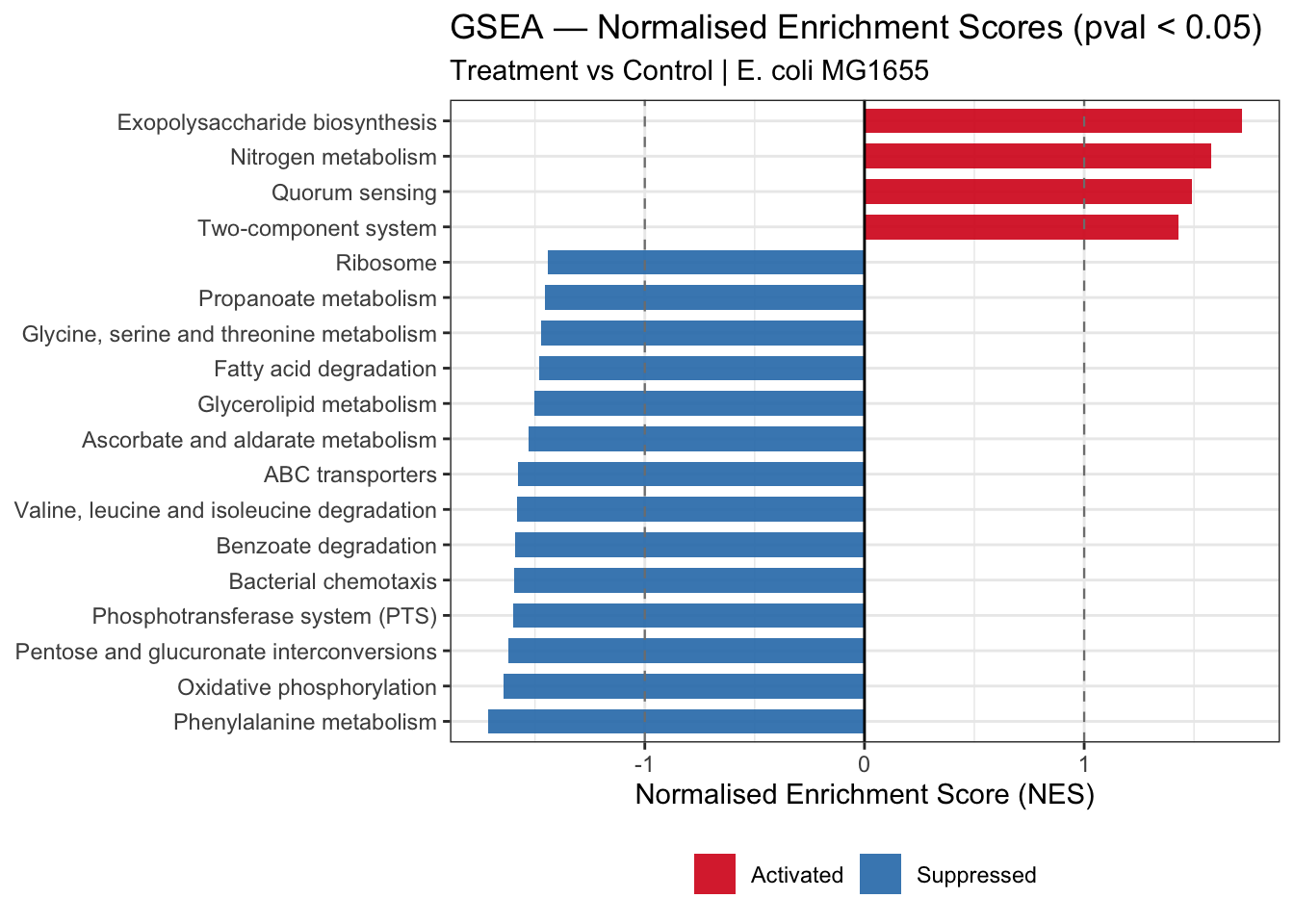

ggplotly(gsea_nesplot)

5.5.6 Dot Plot — NES, padj and Gene Set Size

gsea_dotplot <- ggplot(gsea_bar,
                       aes(x     = NES,
                           y     = pathway,
                           size  = size,
                           color = padj)) +
  geom_point(alpha = 0.85) +
  geom_vline(xintercept = 0, linetype = "dashed", color = "grey50") +
  scale_color_gradient(low = "#CA0020", high = "#92C5DE", name = "padj") +
  scale_size_continuous(name = "Genes in set", range = c(3, 10)) +
  theme_bw() +
  theme(legend.position = "right") +
  labs(
    title    = "GSEA — Pathway Dot Plot",
    subtitle = "Point size = genes in set | Colour = padj",
    x        = "NES",
    y        = NULL
  )

gsea_dotplot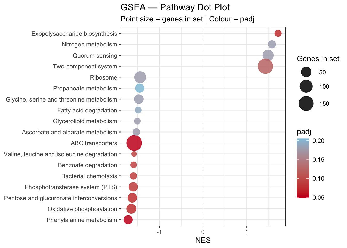

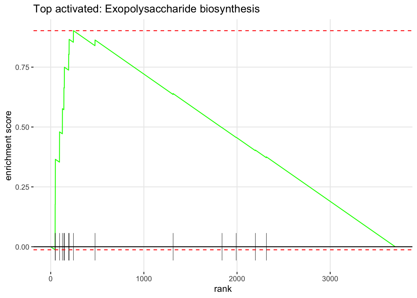
ggplotly(gsea_dotplot)

5.5.7 Enrichment Plot — Top Pathways

The enrichment plot shows the running sum of the enrichment score for a single pathway across the ranked gene list. The peak of the curve is the enrichment score. Genes from the pathway are shown as vertical bars (the “rug”) at the bottom.

# Top activated pathway
top_up <- gsea_results %>%
  as.data.frame() %>%
  filter(NES > 0) %>%
  slice_min(pval, n = 1) %>%
  pull(pathway)

# Top suppressed pathway
top_down <- gsea_results %>%
  as.data.frame() %>%
  filter(NES < 0) %>%
  slice_min(pval, n = 1) %>%
  pull(pathway)

if (length(top_up) > 0) {
  plotEnrichment(pathways_list[[top_up]], rank_vector) +
    labs(title = paste("Top activated:", top_up))
}

if (length(top_down) > 0) {
  plotEnrichment(pathways_list[[top_down]], rank_vector) +
    labs(title = paste("Top suppressed:", top_down))
}