2.13 Adding a smoother to a plot

If you have a scatterplot with a lot of noise, it can be hard to see the dominant pattern.

In this case it’s useful to add a smoothed line to the plot with geom_smooth():

ggplot(mpg, aes(displ, hwy)) + 
  geom_point() + 
  geom_smooth()

## `geom_smooth()` using method = 'loess' and formula = 'y ~ x'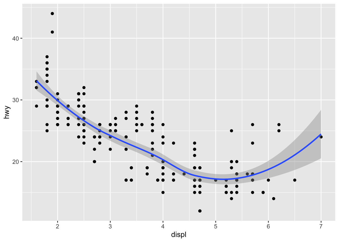

This overlays the scatterplot with a smooth curve, including an assessment of uncertainty in the form of point-wise confidence intervals shown in grey.

If you’re not interested in the confidence interval, turn it off with geom_smooth(se = FALSE).

An important argument to geom_smooth() is the method, which allows you to choose which type of model is used to fit the smooth curve:

method = "loess", the default for small n, uses a smooth local regression.

The wiggliness of the line is controlled by the span parameter, which ranges from 0 (exceedingly wiggly) to 1 (not so wiggly).
```
ggplot(mpg, aes(displ, hwy)) + 
  geom_point() + 
  geom_smooth(span = 0.2)
```
```
## `geom_smooth()` using method = 'loess' and formula = 'y ~ x'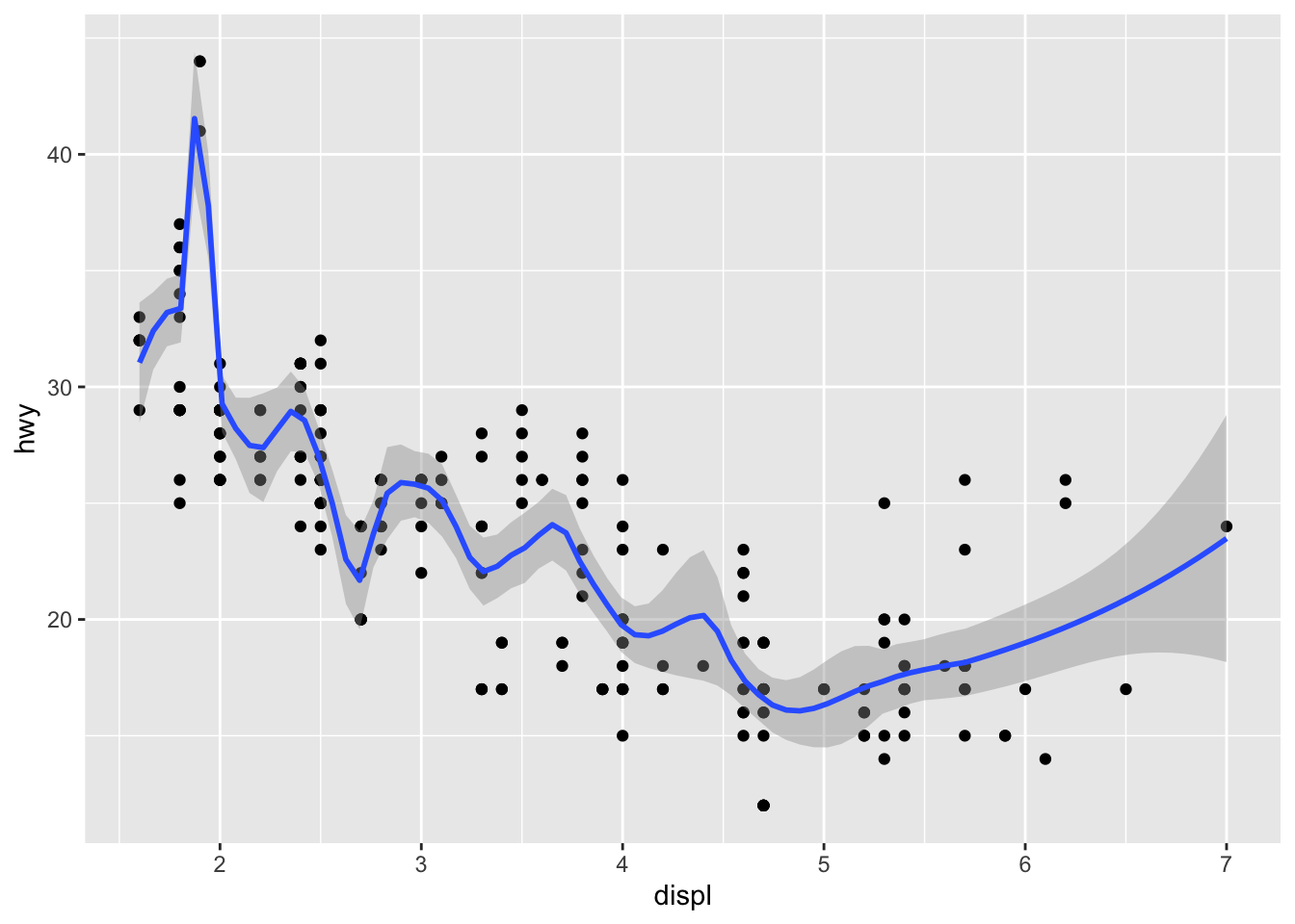
```
```
ggplot(mpg, aes(displ, hwy)) + 
  geom_point() + 
  geom_smooth(span = 1)
```
```
## `geom_smooth()` using method = 'loess' and formula = 'y ~ x'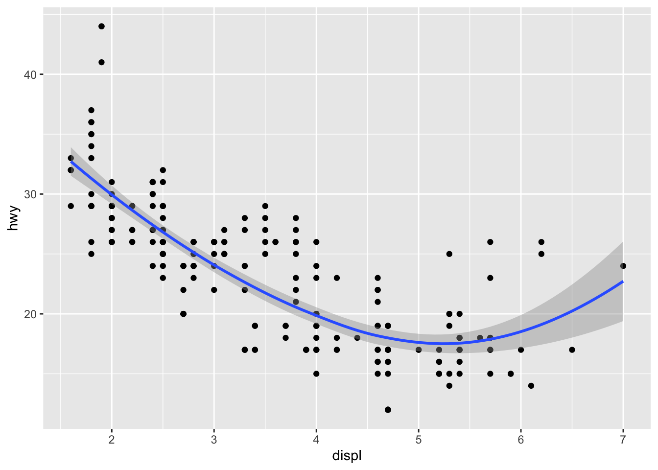
```
Loess does not work well for large datasets (it’s \(O(n^2)\) in memory), so an alternative smoothing algorithm is used when \(n\) is greater than 1,000.
method = "gam" fits a generalised additive model provided by the mgcv package.

You need to first load mgcv, then use a formula like formula = y ~ s(x) or y ~ s(x, bs = "cs") (for large data).

This is what ggplot2 uses when there are more than 1,000 points.
```
library(mgcv)
ggplot(mpg, aes(displ, hwy)) + 
  geom_point() + 
  geom_smooth(method = "gam", formula = y ~ s(x))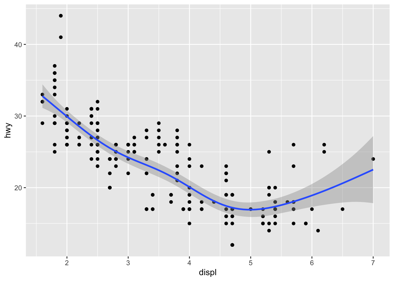
```
method = "lm" fits a linear model, giving the line of best fit.

❓ Question: Can you make a plot using “lm”?

## `geom_smooth()` using formula = 'y ~ x'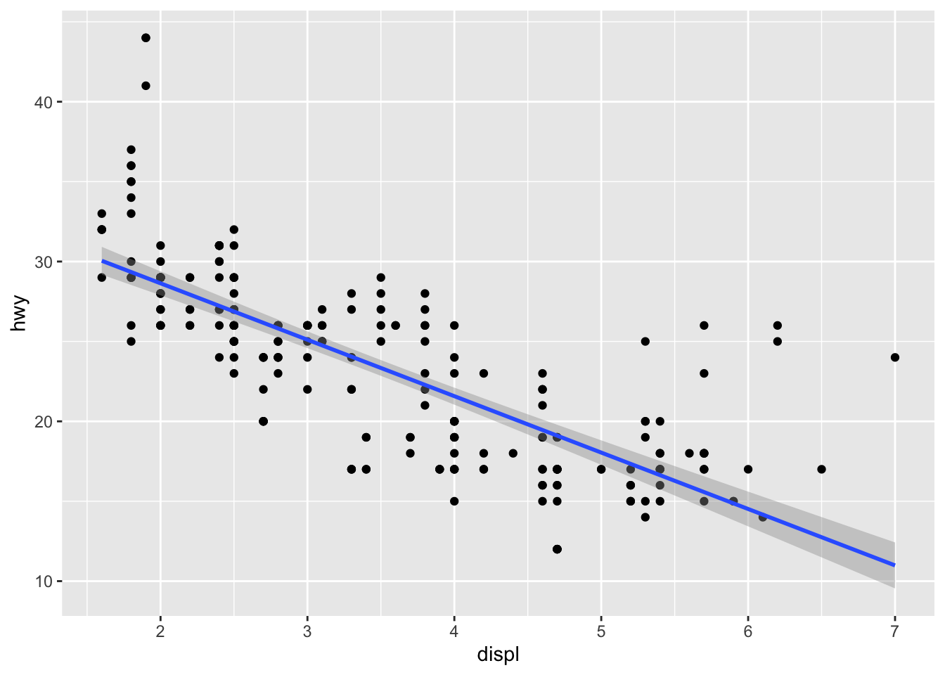

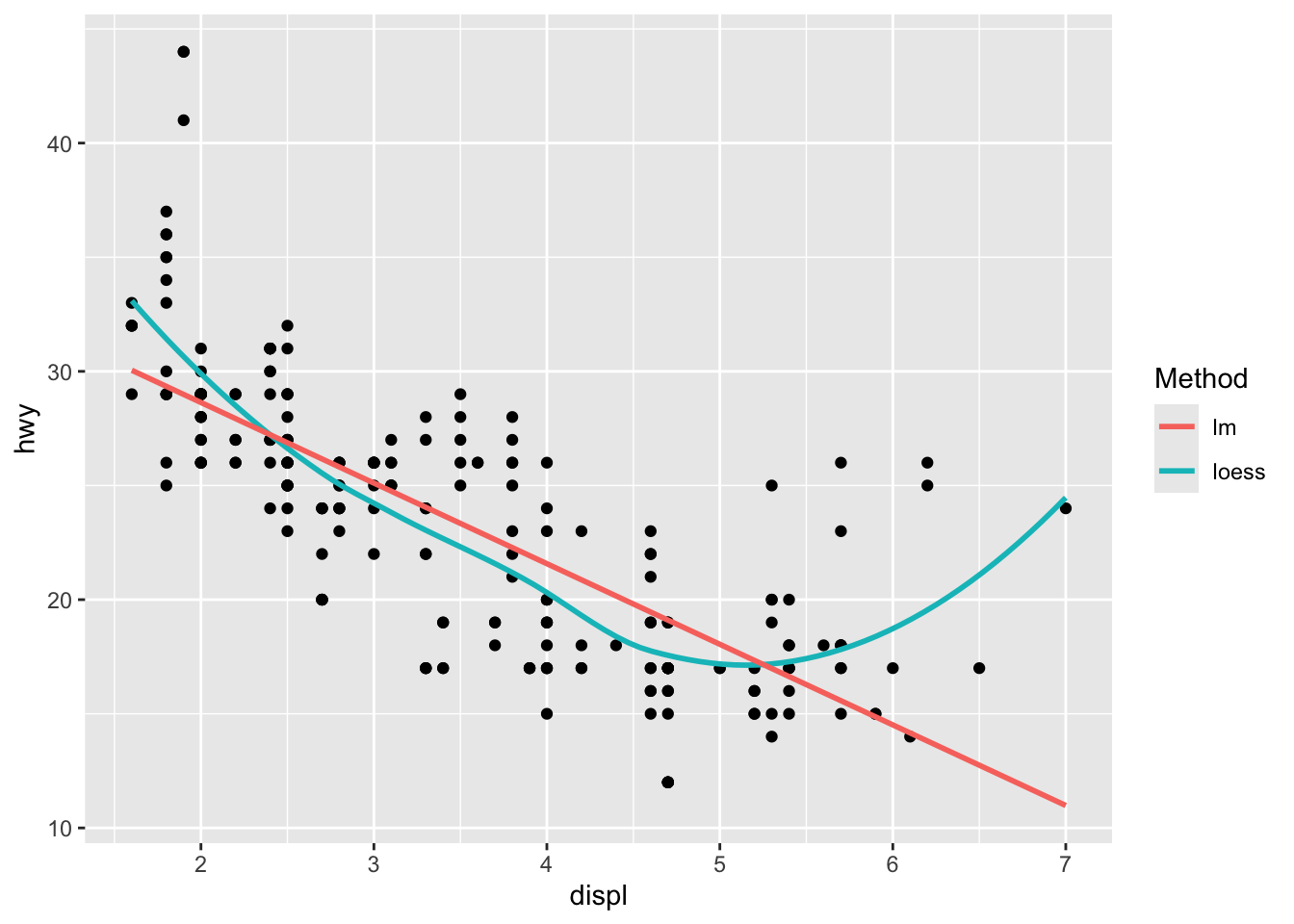
2.13.1 Combining

ggplot(mpg, aes(displ, hwy)) + 
  geom_point() +
  geom_smooth(aes(colour = "loess"), method = "loess", se = FALSE) + 
  geom_smooth(aes(colour = "lm"), method = "lm", se = FALSE) +
  labs(colour = "Method")

## `geom_smooth()` using formula = 'y ~ x'
## `geom_smooth()` using formula = 'y ~ x'